br2

Coefficient of determination (r2) multiplied by the slope of the regression line between sim and obs, with treatment of missing values.

Usage

br2(sim, obs, ...)

# Default S3 method
br2(sim, obs, na.rm=TRUE, use.abs=FALSE, fun=NULL, ..., 
             epsilon.type=c("none", "Pushpalatha2012", "otherFactor", "otherValue"), 
             epsilon.value=NA)

# S3 method for class 'data.frame'
br2(sim, obs, na.rm=TRUE, use.abs=FALSE, fun=NULL, ..., 
             epsilon.type=c("none", "Pushpalatha2012", "otherFactor", "otherValue"), 
             epsilon.value=NA)

# S3 method for class 'matrix'
br2(sim, obs, na.rm=TRUE, use.abs=FALSE, fun=NULL, ..., 
             epsilon.type=c("none", "Pushpalatha2012", "otherFactor", "otherValue"), 
             epsilon.value=NA)

# S3 method for class 'zoo'
br2(sim, obs, na.rm=TRUE, use.abs=FALSE, fun=NULL, ..., 
             epsilon.type=c("none", "Pushpalatha2012", "otherFactor", "otherValue"), 
             epsilon.value=NA)

Arguments

sim

numeric, zoo, matrix or data.frame with simulated values

obs

numeric, zoo, matrix or data.frame with observed values

na.rm

logical value indicating whether 'NA' should be stripped before the computation proceeds.
When an 'NA' value is found at the i-th position in obs OR sim, the i-th value of obs AND sim are removed before the computation.

use.abs

logical value indicating whether the condition to select the formula used to compute br2 should be 'b<=1' or 'abs(b) <=1'.
Krausse et al. (2005) uses 'b<=1' as condition, but strictly speaking this condition should be 'abs(b)<=1'. However, if your model simulations are somewhat "close" to the observations, this condition should not have much impact on the computation of 'br2'.
This argument was introduced in hydroGOF 0.4-0, following a comment by E. White. Its default value is FALSE to ensure compatibility with previous versions of hydroGOF.

fun

function to be applied to sim and obs in order to obtain transformed values thereof before computing this goodness-of-fit index.

The first argument MUST BE a numeric vector with any name (e.g., x), and additional arguments are passed using ....

...

arguments passed to fun, in addition to the mandatory first numeric vector.

epsilon.type

argument used to define a numeric value to be added to both sim and obs before applying fun.

It is was designed to allow the use of logarithm and other similar functions that do not work with zero values.

Valid values of epsilon.type are:

1) "none": sim and obs are used by fun without the addition of any numeric value. This is the default option.

2) "Pushpalatha2012": one hundredth (1/100) of the mean observed values is added to both sim and obs before applying fun, as described in Pushpalatha et al. (2012).

3) "otherFactor": the numeric value defined in the epsilon.value argument is used to multiply the the mean observed values, instead of the one hundredth (1/100) described in Pushpalatha et al. (2012). The resulting value is then added to both sim and obs, before applying fun.

4) "otherValue": the numeric value defined in the epsilon.value argument is directly added to both sim and obs, before applying fun.

epsilon.value

-) when epsilon.type="otherValue" it represents the numeric value to be added to both sim and obs before applying fun.
-) when epsilon.type="otherFactor" it represents the numeric factor used to multiply the mean of the observed values, instead of the one hundredth (1/100) described in Pushpalatha et al. (2012). The resulting value is then added to both sim and obs before applying fun.

Details

$$ br2 = |b| R2 , b <= 1 ; br2 = \frac{R2}{|b|}, b > 1 $$

A model that systematically over or under-predicts all the time will still result in "good" R2 (close to 1), even if all predictions were wrong (Krause et al., 2005). The br2 coefficient allows accounting for the discrepancy in the magnitude of two signals (depicted by 'b') as well as their dynamics (depicted by R2)

Value

br2 between sim and obs.

If sim and obs are matrixes, the returned value is a vector, with the br2 between each column of sim and obs.

References

Krause, P.; Boyle, D.P.; Base, F. (2005). Comparison of different efficiency criteria for hydrological model assessment, Advances in Geosciences, 5, 89-97. doi:10.5194/adgeo-5-89-2005.

Krstic, G.; Krstic, N.S.; Zambrano-Bigiarini, M. (2016). The br2-weighting Method for Estimating the Effects of Air Pollution on Population Health. Journal of Modern Applied Statistical Methods, 15(2), 42. doi:10.22237/jmasm/1478004000

Author

Mauricio Zambrano Bigiarini <mzb.devel@gmail.com>

Note

obs and sim has to have the same length/dimension

The missing values in obs and sim are removed before the computation proceeds, and only those positions with non-missing values in obs and sim are considered in the computation

The slope b is computed as the coefficient of the linear regression between sim and obs, forcing the intercept be equal to zero.

See also

R2, rPearson, rSpearman, cor, lm, gof, ggof

Examples

##################
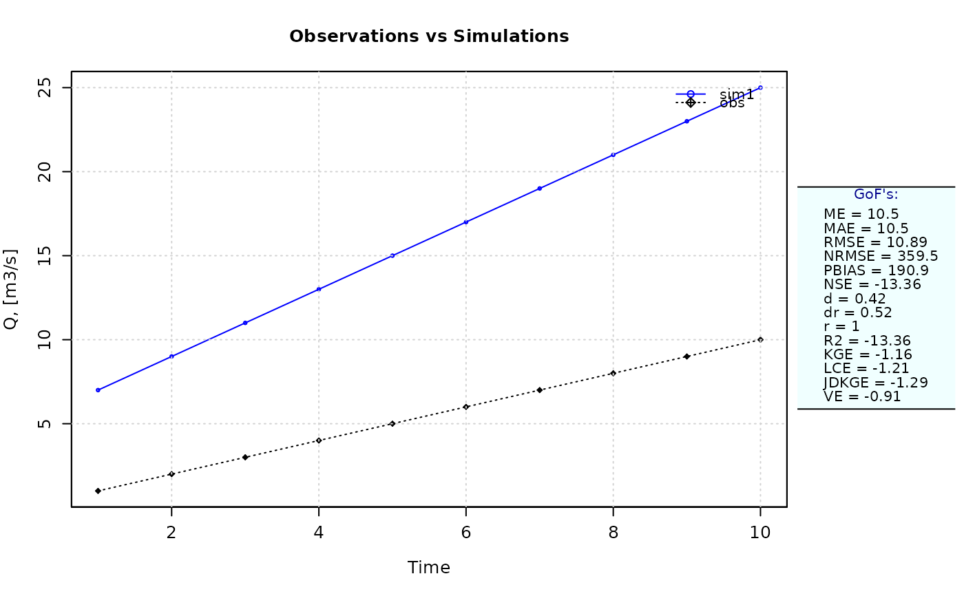
# Example 1: 
# Looking at the difference between r2 and br2 for a case with systematic 
# over-prediction of observed values
obs <- 1:10
sim1 <- 2*obs + 5
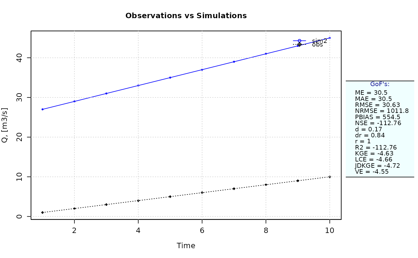
sim2 <- 2*obs + 25

# The coefficient of determination is equal to 1 even if there is no one single 
# simulated value equal to its corresponding observed counterpart
r2 <- (cor(sim1, obs, method="pearson"))^2 # r2=1

# 'br2' effectively penalises the systematic over-estimation
br2(sim1, obs) # br2 = 0.3684211
#> [1] -4.923445
br2(sim2, obs) # br2 = 0.1794872
#> [1] -20.23854

ggof(sim1, obs)
#> [ Note: You did not provide dates, so only a numeric index will be used in the time axis ]

ggof(sim2, obs)
#> [ Note: You did not provide dates, so only a numeric index will be used in the time axis ]


# Computing 'br2' without forcing the intercept be equal to zero
br2.2 <- r2/2 # br2 = 0.5

##################
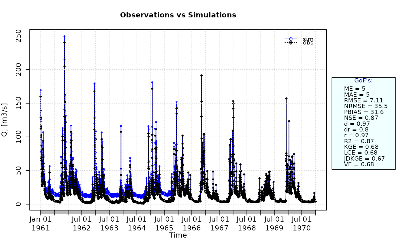
# Example 2: 
# Loading daily streamflows of the Ega River (Spain), from 1961 to 1970
data(EgaEnEstellaQts)
obs <- EgaEnEstellaQts

# Generating a simulated daily time series, initially equal to the observed series
sim <- obs 

# Computing the 'br2' for the "best" (unattainable) case
br2(sim=sim, obs=obs)
#> [1] 1

##################
# Example 3: br2 for simulated values equal to observations plus random noise 
#            on the first half of the observed values. 
#            This random noise has more relative importance for ow flows than 
#            for medium and high flows.
  
# Randomly changing the first 1826 elements of 'sim', by using a normal distribution 
# with mean 10 and standard deviation equal to 1 (default of 'rnorm').
sim[1:1826] <- obs[1:1826] + rnorm(1826, mean=10)
ggof(sim, obs)


br2(sim=sim, obs=obs)
#> [1] 0.7775568

##################
# Example 4: br2 for simulated values equal to observations plus random noise 
#            on the first half of the observed values and applying (natural) 
#            logarithm to 'sim' and 'obs' during computations.

br2(sim=sim, obs=obs, fun=log)
#> [1] 0.4295402

# Verifying the previous value:
lsim <- log(sim)
lobs <- log(obs)
br2(sim=lsim, obs=lobs)
#> [1] 0.4295402

##################
# Example 5: br2 for simulated values equal to observations plus random noise 
#            on the first half of the observed values and applying (natural) 
#            logarithm to 'sim' and 'obs' and adding the Pushpalatha2012 constant
#            during computations

br2(sim=sim, obs=obs, fun=log, epsilon.type="Pushpalatha2012")
#> [1] 0.4362199

# Verifying the previous value, with the epsilon value following Pushpalatha2012
eps  <- mean(obs, na.rm=TRUE)/100
lsim <- log(sim+eps)
lobs <- log(obs+eps)
br2(sim=lsim, obs=lobs)
#> [1] 0.4362199

##################
# Example 6: br2 for simulated values equal to observations plus random noise 
#            on the first half of the observed values and applying (natural) 
#            logarithm to 'sim' and 'obs' and adding a user-defined constant
#            during computations

eps <- 0.01
br2(sim=sim, obs=obs, fun=log, epsilon.type="otherValue", epsilon.value=eps)
#> [1] 0.4299742

# Verifying the previous value:
lsim <- log(sim+eps)
lobs <- log(obs+eps)
br2(sim=lsim, obs=lobs)
#> [1] 0.4299742

##################
# Example 7: br2 for simulated values equal to observations plus random noise 
#            on the first half of the observed values and applying (natural) 
#            logarithm to 'sim' and 'obs' and using a user-defined factor
#            to multiply the mean of the observed values to obtain the constant
#            to be added to 'sim' and 'obs' during computations

fact <- 1/50
br2(sim=sim, obs=obs, fun=log, epsilon.type="otherFactor", epsilon.value=fact)
#> [1] 0.4425449

# Verifying the previous value:
eps  <- fact*mean(obs, na.rm=TRUE)
lsim <- log(sim+eps)
lobs <- log(obs+eps)
br2(sim=lsim, obs=lobs)
#> [1] 0.4425449

##################
# Example 8: br2 for simulated values equal to observations plus random noise 
#            on the first half of the observed values and applying a 
#            user-defined function to 'sim' and 'obs' during computations

fun1 <- function(x) {sqrt(x+1)}

br2(sim=sim, obs=obs, fun=fun1)
#> [1] 0.6475741

# Verifying the previous value, with the epsilon value following Pushpalatha2012
sim1 <- sqrt(sim+1)
obs1 <- sqrt(obs+1)
br2(sim=sim1, obs=obs1)
#> [1] 0.6475741