Goodness-of-fit measures to compare observed and simulated time series with hydroGOF

Citation

If you use hydroGOF, please cite it as Zambrano-Bigiarini (2026):

Zambrano-Bigiarini, M. (2026) hydroGOF: Goodness-of-fit functions for comparison of simulated and observed hydrological time series R package version 0.7-0. URL: https://cran.r-project.org/package=hydroGOF. doi:10.32614/CRAN.package.hydroGOF.

Installation

Installing the latest stable version (from CRAN):

install.packages("hydroGOF")

Alternatively, you can also try the under-development version (from Github):

if (!require(devtools)) install.packages("devtools")
library(devtools)
install_github("hzambran/hydroGOF")

Setting up the environment

Loading the hydroGOF package, which contains data and functions used in this analysis:

library(hydroGOF)

## Loading required package: zoo

## 
## Attaching package: 'zoo'

## The following objects are masked from 'package:base':
## 
##     as.Date, as.Date.numeric

Example using NSE

The following examples use the well-known Nash-Sutcliffe efficiency (NSE), but you can repeat the computations using any of the goodness-of-fit measures included in the hydroGOF package (e.g., KGE, ubRMSE, dr).

Ex 1: ideal integer values

Basic ideal case with a numeric sequence of integers:

obs <- 1:10
sim <- 1:10
NSE(sim, obs)

## [1] 1

obs <- 1:10
sim <- 2:11
NSE(sim, obs)

## [1] 0.8787879

Ex 2: ideal real values

Basic ideal case with a numeric sequence of integers:

obs <- 1:10 + 0.1
sim <- 1:10 +0.1
NSE(sim, obs)

## [1] 1

obs <- 1:10 + 0.1
sim <- 2:11 + 0.1
NSE(sim, obs)

## [1] 0.8787879

Ex 3: ideal daily ts

From this example onwards, a streamflow time series will be used.

First, we load the daily streamflows of the Ega River (Spain), from 1961 to 1970:

data(EgaEnEstellaQts)
obs <- EgaEnEstellaQts

Generating a simulated daily time series, initially equal to the observed series:

sim <- obs

Visualising the observed and simulated time series:

ggof(sim, obs)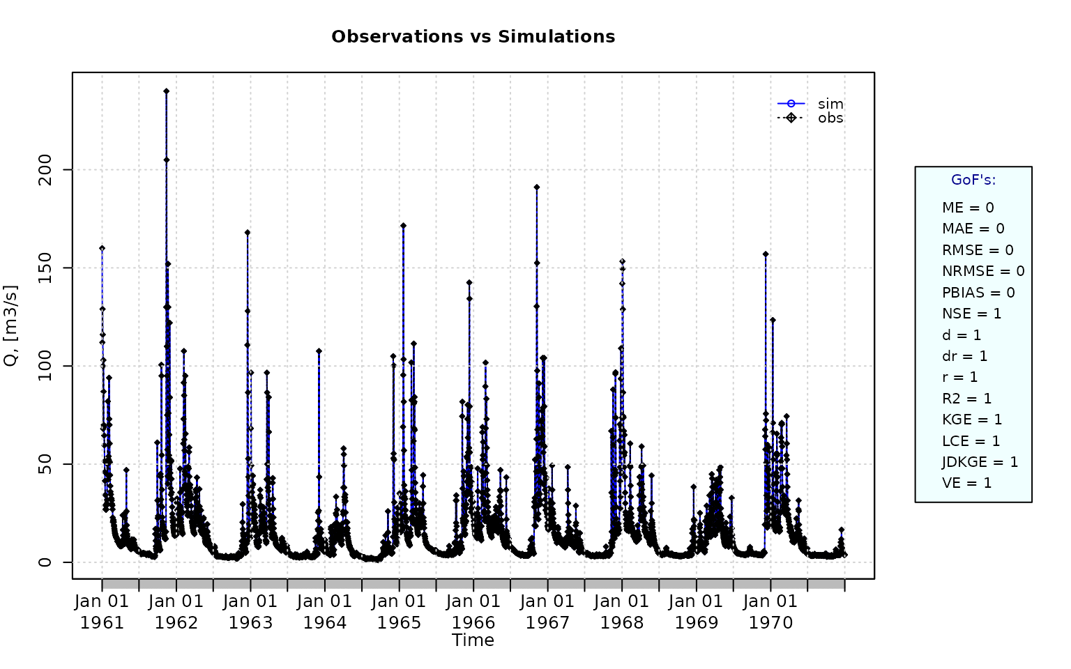

Computing the ‘NSE’ for the “best” (unattainable) case

NSE(sim=sim, obs=obs)

## [1] 1

Ex 4: random noise in the first half of the simulated values

NSE for simulated values equal to observations plus random noise on the first half of the observed values.

This random noise has more relative importance for low flows than for medium and high flows.

Randomly changing the first 1826 elements of ‘sim’, by using a normal distribution with mean 10 and standard deviation equal to 1 (default of ‘rnorm’).

sim[1:1826] <- obs[1:1826] + rnorm(1826, mean=10)
ggof(sim, obs)

NSE(sim=sim, obs=obs)

## [1] 0.8739885

Let’s have a look at other goodness-of-fit measures:

mNSE(sim=sim, obs=obs)                 # Modified NSE

## [1] 0.6049584

rNSE(sim=sim, obs=obs)                 # Relative NSE

## [1] -0.5687206

wNSE(sim=sim, obs=obs)                 # Weighted NSE

## [1] 0.9769178

wsNSE(sim=sim, obs=obs)                # Weighted Seasonal NSE

## [1] 0.9686072

KGE(sim=sim, obs=obs)                  # Kling-Gupta efficiency (KGE), 2009

## [1] 0.6805856

KGE(sim=sim, obs=obs, method="2012")   # Kling-Gupta efficiency (KGE), 2012

## [1] 0.61689

KGE(sim=sim, obs=obs, method="2021")   # Kling-Gupta efficiency (KGE), 2021

## [1] 0.7461172

KGElf(sim=sim, obs=obs)                # KGE for low flows

## [1] 0.5170138

KGEnp(sim=sim, obs=obs)                # Non-parametric KGE

## [1] 0.6340134

sKGE(sim=sim, obs=obs)                 # Split KGE

## [1] 0.6547522

KGEkm(sim=sim, obs=obs)                # Knowable Moments KGE

## [1] 0.6467934

JDKGE(sim=sim, obs=obs)                # Joint Divergence KGE

## [1] 0.6080188

d(sim=sim, obs=obs)                    # Index of Agreement

## [1] 0.9697286

dr(sim=sim, obs=obs)                   # Refined Index of Agreement

## [1] 0.8024792

md(sim=sim, obs=obs)                   # Modified Index of Agreement

## [1] 0.7980307

rd(sim=sim, obs=obs)                   # Relative Index of Agreement

## [1] 0.6231506

VE(sim=sim, obs=obs)                   # Volumetric Efficiency

## [1] 0.6838531

cp(sim=sim, obs=obs)                   # Coefficient of Persistence

## [1] 0.4683536

APFB(sim=sim, obs=obs)                 # Annual Peak Flow Bias

## [1] 0.03202514

HFB(sim=sim, obs=obs)                  # High Flow Bias

## [1] 0.08706977

LME(sim=sim, obs=obs)                  # Liu-Mean Efficiency

## [1] 0.6838398

LCE(sim=sim, obs=obs)                  # Lee and Choi Efficiency

## [1] 0.6777786

PMR(sim=sim, obs=obs)                  # Proxy for Model Robustness

## [1] 0.3156247

pbias(sim=sim, obs=obs)                # Percent bias (PBIAS)

## [1] 31.6

pbiasfdc(sim=sim, obs=obs)             # PBIAS in the slope of the midsegment of the FDC

## [Note: 'thr.shw' was set to FALSE to avoid confusing legends...]

## [1] -34.95419

me(sim=sim, obs=obs)                   # Mean Error

## [1] 4.998998

mae(sim=sim, obs=obs)                  # Mean Absolute Error

## [1] 4.998998

mse(sim=sim, obs=obs)                  # Mean Squared Error

## [1] 50.46771

rmse(sim=sim, obs=obs)                 # Root Mean Square Error (RMSE)

## [1] 7.104063

ubRMSE(sim=sim, obs=obs)               # Unbiased RMSE

## [1] 5.047547

nrmse(sim=sim, obs=obs, norm="sd")     # Normalised Root Mean Square Error

## [1] 35.5

nrmse(sim=sim, obs=obs, norm="maxmin") # Normalised Root Mean Square Error

## [1] 3

nrmse(sim=sim, obs=obs, norm="mean")   # Normalised Root Mean Square Error

## [1] 44.9

nrmse(sim=sim, obs=obs, norm="IQR")    # Normalised Root Mean Square Error

## [1] 47.1

rPearson(sim=sim, obs=obs)             # Pearson correlation coefficient

## [1] 0.9698058

rSpearman(sim=sim, obs=obs)            # Spearman rank correlation coefficient

## [1] 0.8362479

R2(sim=sim, obs=obs)                   # Coefficient of determination (R2)

## [1] 0.8739885

br2(sim=sim, obs=obs)                  # R2 multiplied by the slope of the regression line

## [1] 0.7780545

Ex 5: random noise and logarithmic transformation

NSE for simulated values equal to observations plus random noise on the first half of the observed values and applying (natural) logarithm to obs against sim during computations.

NSE(sim=sim, obs=obs, fun=log)

## [1] 0.4799297

Verifying the previous value:

lsim <- log(sim)
lobs <- log(obs)
NSE(sim=lsim, obs=lobs)

## [1] 0.4799297

Let’s have a look at other goodness-of-fit measures:

mNSE(sim=sim, obs=obs)                 # Modified NSE

## [1] 0.6049584

rNSE(sim=sim, obs=obs)                 # Relative NSE

## [1] -0.5687206

wNSE(sim=sim, obs=obs)                 # Weighted NSE

## [1] 0.9769178

wsNSE(sim=sim, obs=obs)                # Weighted Seasonal NSE

## [1] 0.9686072

KGE(sim=sim, obs=obs)                  # Kling-Gupta efficiency (KGE), 2009

## [1] 0.6805856

KGE(sim=sim, obs=obs, method="2012")   # Kling-Gupta efficiency (KGE), 2012

## [1] 0.61689

KGE(sim=sim, obs=obs, method="2021")   # Kling-Gupta efficiency (KGE), 2021

## [1] 0.7461172

KGElf(sim=sim, obs=obs)                # KGE for low flows

## [1] 0.5170138

KGEnp(sim=sim, obs=obs)                # Non-parametric KGE

## [1] 0.6340134

sKGE(sim=sim, obs=obs)                 # Split KGE

## [1] 0.6547522

KGEkm(sim=sim, obs=obs)                # Knowable Moments KGE

## [1] 0.6467934

JDKGE(sim=sim, obs=obs)                # Joint Divergence KGE

## [1] 0.6080188

d(sim=sim, obs=obs)                    # Index of Agreement

## [1] 0.9697286

dr(sim=sim, obs=obs)                   # Refined Index of Agreement

## [1] 0.8024792

md(sim=sim, obs=obs)                   # Modified Index of Agreement

## [1] 0.7980307

rd(sim=sim, obs=obs)                   # Relative Index of Agreement

## [1] 0.6231506

VE(sim=sim, obs=obs)                   # Volumetric Efficiency

## [1] 0.6838531

cp(sim=sim, obs=obs)                   # Coefficient of Persistence

## [1] 0.4683536

APFB(sim=sim, obs=obs)                 # Annual Peak Flow Bias

## [1] 0.03202514

HFB(sim=sim, obs=obs)                  # High Flow Bias

## [1] 0.08706977

LME(sim=sim, obs=obs)                  # Liu-Mean Efficiency

## [1] 0.6838398

LCE(sim=sim, obs=obs)                  # Lee and Choi Efficiency

## [1] 0.6777786

PMR(sim=sim, obs=obs)                  # Proxy for Model Robustness

## [1] 0.3156247

pbias(sim=sim, obs=obs)                # Percent bias (PBIAS)

## [1] 31.6

pbiasfdc(sim=sim, obs=obs)             # PBIAS in the slope of the midsegment of the FDC

## [Note: 'thr.shw' was set to FALSE to avoid confusing legends...]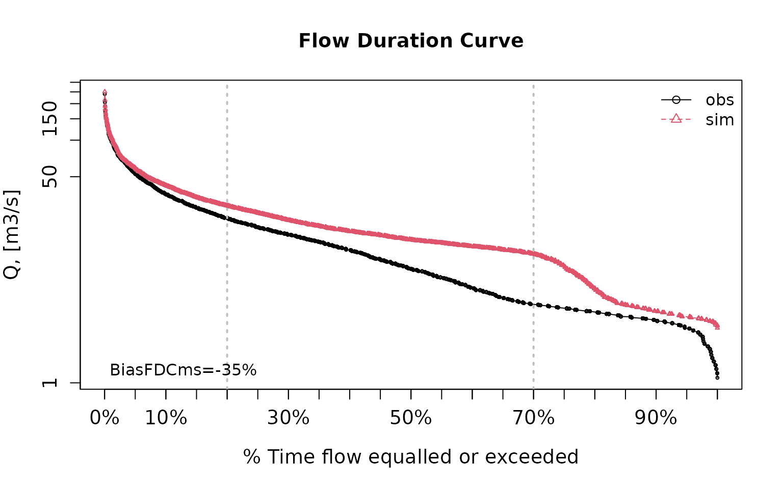

## [1] -34.95419

me(sim=sim, obs=obs)                   # Mean Error

## [1] 4.998998

mae(sim=sim, obs=obs)                  # Mean Absolute Error

## [1] 4.998998

mse(sim=sim, obs=obs)                  # Mean Squared Error

## [1] 50.46771

rmse(sim=sim, obs=obs)                 # Root Mean Square Error (RMSE)

## [1] 7.104063

ubRMSE(sim=sim, obs=obs)               # Unbiased RMSE

## [1] 5.047547

nrmse(sim=sim, obs=obs, norm="sd")     # Normalised Root Mean Square Error

## [1] 35.5

nrmse(sim=sim, obs=obs, norm="maxmin") # Normalised Root Mean Square Error

## [1] 3

nrmse(sim=sim, obs=obs, norm="mean")   # Normalised Root Mean Square Error

## [1] 44.9

nrmse(sim=sim, obs=obs, norm="IQR")    # Normalised Root Mean Square Error

## [1] 47.1

rPearson(sim=sim, obs=obs)             # Pearson correlation coefficient

## [1] 0.9698058

rSpearman(sim=sim, obs=obs)            # Spearman rank correlation coefficient

## [1] 0.8362479

R2(sim=sim, obs=obs)                   # Coefficient of determination (R2)

## [1] 0.8739885

br2(sim=sim, obs=obs)                  # R2 multiplied by the slope of the regression line

## [1] 0.7780545

Ex 6: random noise, logarithmic transformation and Pushpalatha2012 constant

NSE for simulated values equal to observations plus random noise on the first half of the observed values and applying (natural) logarithm to obs against sim and adding the Pushpalatha2012 constant during computations.

NSE(sim=sim, obs=obs, fun=log, epsilon.type="Pushpalatha2012")

## [1] 0.4871177

Verifying the previous value, with the epsilon value following Pushpalatha2012:

eps  <- mean(obs, na.rm=TRUE)/100
lsim <- log(sim+eps)
lobs <- log(obs+eps)
NSE(sim=lsim, obs=lobs)

## [1] 0.4871177

Let’s have a look at other goodness-of-fit measures:

gof(sim=sim, obs=obs, fun=log, epsilon.type="Pushpalatha2012", do.spearman=TRUE, do.pbfdc=TRUE, do.pmr=TRUE)

##              [,1]
## ME           0.41
## MAE          0.41
## MSE          0.46
## RMSE         0.68
## ubRMSE       0.54
## NRMSE %     71.60
## PBIAS %     18.20
## RSR          0.72
## rSD          0.89
## NSE          0.49
## mNSE         0.48
## rNSE        -2.08
## wNSE         0.74
## wsNSE        0.78
## d            0.86
## dr           0.74
## md           0.74
## rd           0.18
## cp          -7.68
## r            0.83
## R2           0.49
## bR2          0.44
## VE           0.82
## KGE          0.72
## KGElf        0.52
## KGEnp        0.74
## KGEkm        0.74
## JDKGE        0.72
## LME          0.68
## LCE          0.67
## sKGE         0.53
## APFB         0.01
## HFB          0.02
## rSpearman    0.84
## pbiasFDC % -45.87
## PMR          0.20

Ex 7: random noise, logarithmic transformation and user-defined constant

NSE for simulated values equal to observations plus random noise on the first half of the observed values and applying (natural) logarithm to obs against sim and adding a user-defined constant during computations

eps <- 0.01
NSE(sim=sim, obs=obs, fun=log, epsilon.type="otherValue", epsilon.value=eps)

## [1] 0.4804

Verifying the previous value:

lsim <- log(sim+eps)
lobs <- log(obs+eps)
NSE(sim=lsim, obs=lobs)

## [1] 0.4804

Let’s have a look at other goodness-of-fit measures:

gof(sim=sim, obs=obs, fun=log, epsilon.type="otherValue", epsilon.value=eps, do.spearman=TRUE, do.pbfdc=TRUE, do.pmr=TRUE)

##              [,1]
## ME           0.42
## MAE          0.42
## MSE          0.48
## RMSE         0.69
## ubRMSE       0.55
## NRMSE %     72.10
## PBIAS %     18.70
## RSR          0.72
## rSD          0.88
## NSE          0.48
## mNSE         0.48
## rNSE        -4.22
## wNSE         0.74
## wsNSE        0.78
## d            0.86
## dr           0.74
## md           0.74
## rd          -0.39
## cp          -7.93
## r            0.82
## R2           0.48
## bR2          0.43
## VE           0.81
## KGE          0.72
## KGElf        0.51
## KGEnp        0.74
## KGEkm        0.73
## JDKGE        0.71
## LME          0.67
## LCE          0.66
## sKGE         0.48
## APFB         0.01
## HFB          0.02
## rSpearman    0.84
## pbiasFDC % -46.36
## PMR          0.21

Ex 8: random noise, logarithmic transformation and user-defined factor

NSE for simulated values equal to observations plus random noise on the first half of the observed values and applying (natural) logarithm to obs against sim and using a user-defined factor to multiply the mean of the observed values to obtain the constant to be added to obs against sim during computations

fact <- 1/50
NSE(sim=sim, obs=obs, fun=log, epsilon.type="otherFactor", epsilon.value=fact)

## [1] 0.4938294

Verifying the previous value:

fact <- 1/50
eps  <- fact*mean(obs, na.rm=TRUE)
lsim <- log(sim+eps)
lobs <- log(obs+eps)
NSE(sim=lsim, obs=lobs)

## [1] 0.4938294

Let’s have a look at other goodness-of-fit measures:

gof(sim=sim, obs=obs, fun=log, epsilon.type="otherFactor", epsilon.value=fact, do.spearman=TRUE, do.pbfdc=TRUE, do.pmr=TRUE)

##              [,1]
## ME           0.41
## MAE          0.41
## MSE          0.44
## RMSE         0.66
## ubRMSE       0.52
## NRMSE %     71.10
## PBIAS %     17.60
## RSR          0.71
## rSD          0.89
## NSE          0.49
## mNSE         0.48
## rNSE        -1.33
## wNSE         0.74
## wsNSE        0.78
## d            0.87
## dr           0.74
## md           0.74
## rd           0.38
## cp          -7.43
## r            0.83
## R2           0.49
## bR2          0.44
## VE           0.82
## KGE          0.73
## KGElf        0.53
## KGEnp        0.74
## KGEkm        0.75
## JDKGE        0.72
## LME          0.68
## LCE          0.68
## sKGE         0.56
## APFB         0.01
## HFB          0.02
## rSpearman    0.84
## pbiasFDC % -45.37
## PMR          0.19

Ex 9: random noise, user-defined transformation

NSE for simulated values equal to observations plus random noise on the first half of the observed values and applying a user-defined function to obs against sim during computations:

fun1 <- function(x) {sqrt(x+1)}
NSE(sim=sim, obs=obs, fun=fun1)

## [1] 0.7265255

Verifying the previous value, with the epsilon value following Pushpalatha2012:

sim1 <- sqrt(sim+1)
obs1 <- sqrt(obs+1)
NSE(sim=sim1, obs=obs1)

## [1] 0.7265255

gof(sim=sim, obs=obs, fun=fun1, do.spearman=TRUE, do.pbfdc=TRUE, do.pmr=TRUE)

##              [,1]
## ME           0.65
## MAE          0.65
## MSE          0.92
## RMSE         0.96
## ubRMSE       0.71
## NRMSE %     52.30
## PBIAS %     17.70
## RSR          0.52
## rSD          0.97
## NSE          0.73
## mNSE         0.54
## rNSE         0.34
## wNSE         0.89
## wsNSE        0.76
## d            0.93
## dr           0.77
## md           0.76
## rd           0.83
## cp          -1.17
## r            0.92
## R2           0.73
## bR2          0.65
## VE           0.82
## KGE          0.81
## KGElf        0.50
## KGEnp        0.75
## KGEkm        0.80
## JDKGE        0.79
## LME          0.80
## LCE          0.79
## sKGE         0.84
## APFB         0.02
## HFB          0.04
## rSpearman    0.84
## pbiasFDC % -32.96
## PMR          0.19

A short example from hydrological modelling

Loading observed streamflows of the Ega River (Spain), with daily data from 1961-Jan-01 up to 1970-Dec-31

require(zoo)
data(EgaEnEstellaQts)
obs <- EgaEnEstellaQts

Generating a simulated daily time series, initially equal to the observed values (simulated values are usually read from the output files of the hydrological model)

sim <- obs

Plotting the graphical comparison of obs against sim, along with the default goodness-of-fit measures:

ggof(sim, obs)

Plotting the graphical comparison of obs against sim, along with user-defined goodness-of-fit measures:

ggof(sim, obs, 
     gofs=c( "PBIAS", "dr", "R2",  "NSE", "KGE",  "LCE", "JDKGE", "APFB", "HFB"))

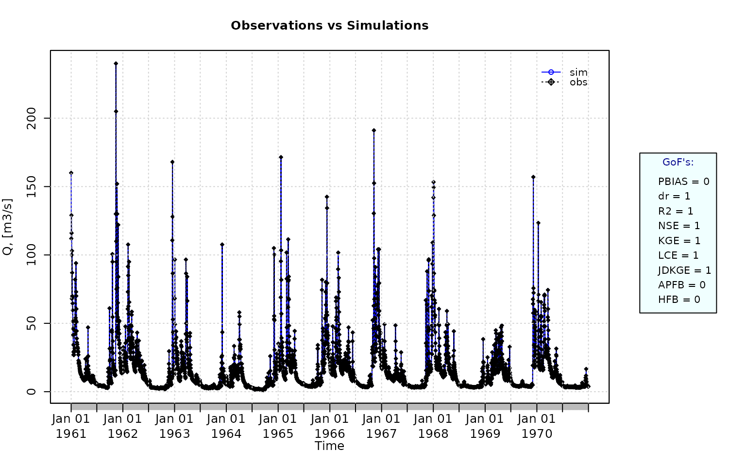
Computing the numeric goodness-of-fit measures for the best (unattainable) case, including the following three measures that -due to slightly high computation time- are not computed by default: i) the Spearman’s Rank Correlation Coefficient (rSpearman), ii) the percent bias in the Slope of the Midsegment of the Flow Duration Curve (pbiasFDC), and iii) the Proxy for Model Robustness (PMR).

gof(sim=sim, obs=obs, do.spearman=TRUE, do.pbfdc=TRUE, do.pmr=TRUE)

##            [,1]
## ME            0
## MAE           0
## MSE           0
## RMSE          0
## ubRMSE        0
## NRMSE %       0
## PBIAS %       0
## RSR           0
## rSD           1
## NSE           1
## mNSE          1
## rNSE          1
## wNSE          1
## wsNSE         1
## d             1
## dr            1
## md            1
## rd            1
## cp            1
## r             1
## R2            1
## bR2           1
## VE            1
## KGE           1
## KGElf         1
## KGEnp         1
## KGEkm         1
## JDKGE         1
## LME           1
## LCE           1
## sKGE          1
## APFB          0
## HFB           0
## rSpearman     1
## pbiasFDC %    0
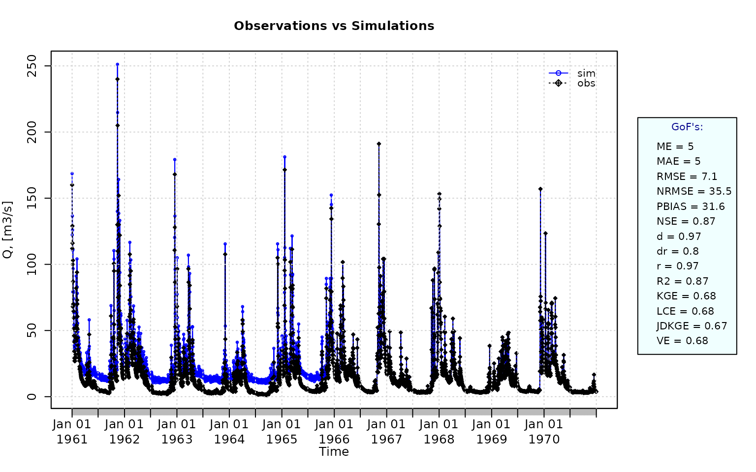
## PMR           0

Randomly changing the first 1826 elements of ‘sim’ (half of the ts), by using a normal distribution with mean 10 and standard deviation equal to 1 (default of ‘rnorm’).

sim[1:1826] <- obs[1:1826] + rnorm(1826, mean=10)

Plotting the graphical comparison of obs against sim, along with the default goodness-of-fit measures for the daily and monthly time series:

ggof(sim=sim, obs=obs, ftype="dm", FUN=mean)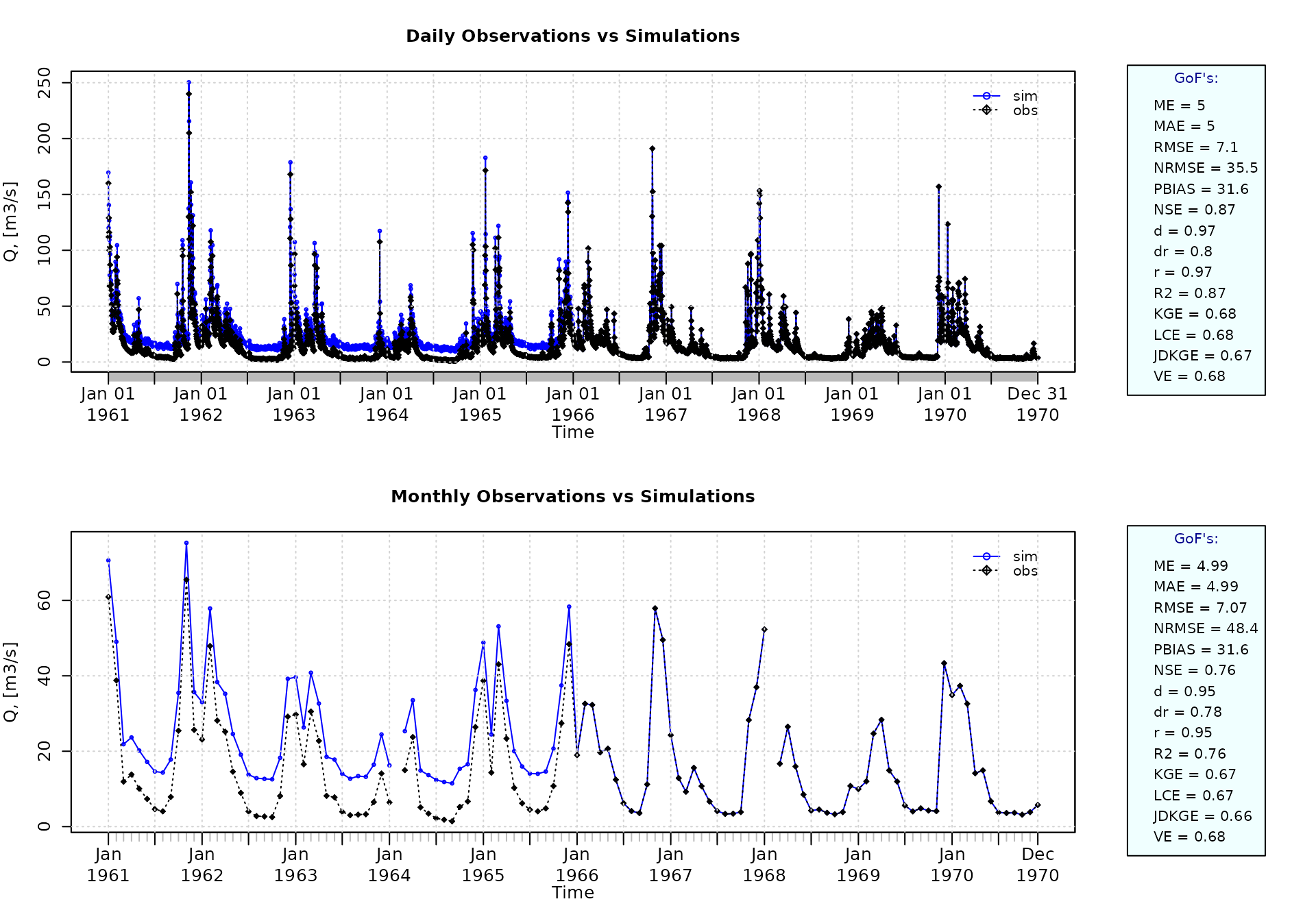

Plotting the graphical comparison of obs against sim, along with user-defined goodness-of-fit measures for the daily and monthly time series:

ggof(sim=sim, obs=obs, ftype="dm", FUN=mean,
     gofs=c( "PBIAS", "dr", "R2",  "NSE", "KGE",  "LCE", "JDKGE", "APFB", "HFB"))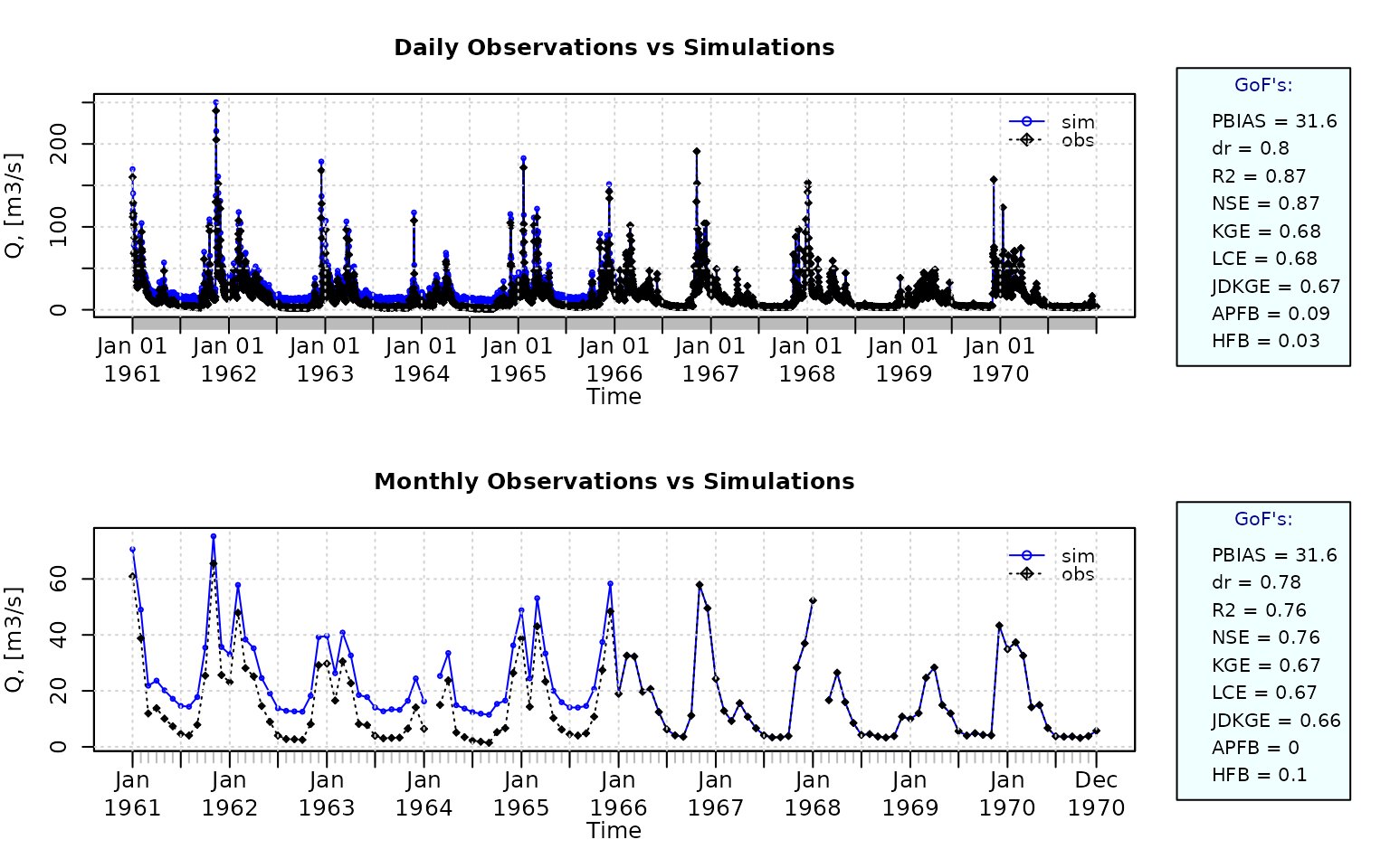

Removing warm-up period

Using the first two years (1961-1962) as warm-up period, and removing the corresponding observed and simulated values from the computation of the goodness-of-fit measures:

ggof(sim=sim, obs=obs, ftype="dm", FUN=mean, cal.ini="1963-01-01")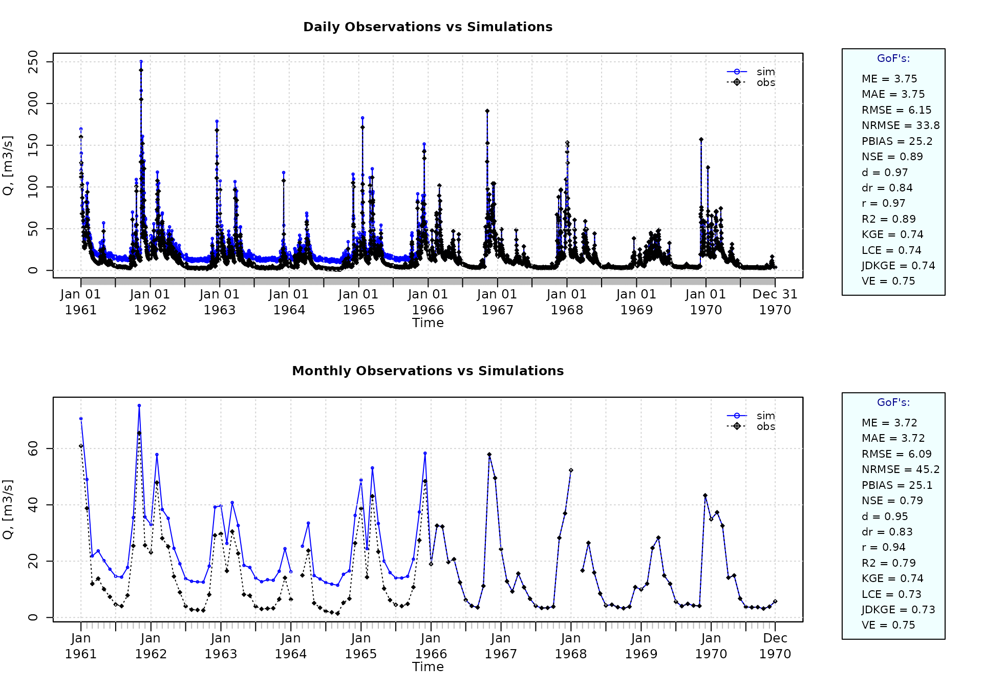

Verification of the goodness-of-fit measures for the daily values after removing the warm-up period:

sim <- window(sim, start="1963-01-01")
obs <- window(obs, start="1963-01-01")

gof(sim, obs)

##          [,1]
## ME       3.75
## MAE      3.75
## MSE     37.84
## RMSE     6.15
## ubRMSE   4.88
## NRMSE % 33.80
## PBIAS % 25.20
## RSR      0.34
## rSD      1.02
## NSE      0.89
## mNSE     0.68
## rNSE    -0.48
## wNSE     0.98
## wsNSE    0.82
## d        0.97
## dr       0.84
## md       0.84
## rd       0.64
## cp       0.52
## r        0.97
## R2       0.89
## bR2      0.81
## VE       0.75
## KGE      0.74
## KGElf    0.57
## KGEnp    0.69
## KGEkm    0.73
## JDKGE    0.74
## LME      0.75
## LCE      0.74
## sKGE     0.70
## APFB     0.03
## HFB      0.00

Plotting uncertainty bands

Generating fictitious lower and upper uncertainty bounds:

lband <- obs - 5
uband <- obs + 5

Plotting the previously generated uncertainty bands:

plotbands(obs, lband, uband)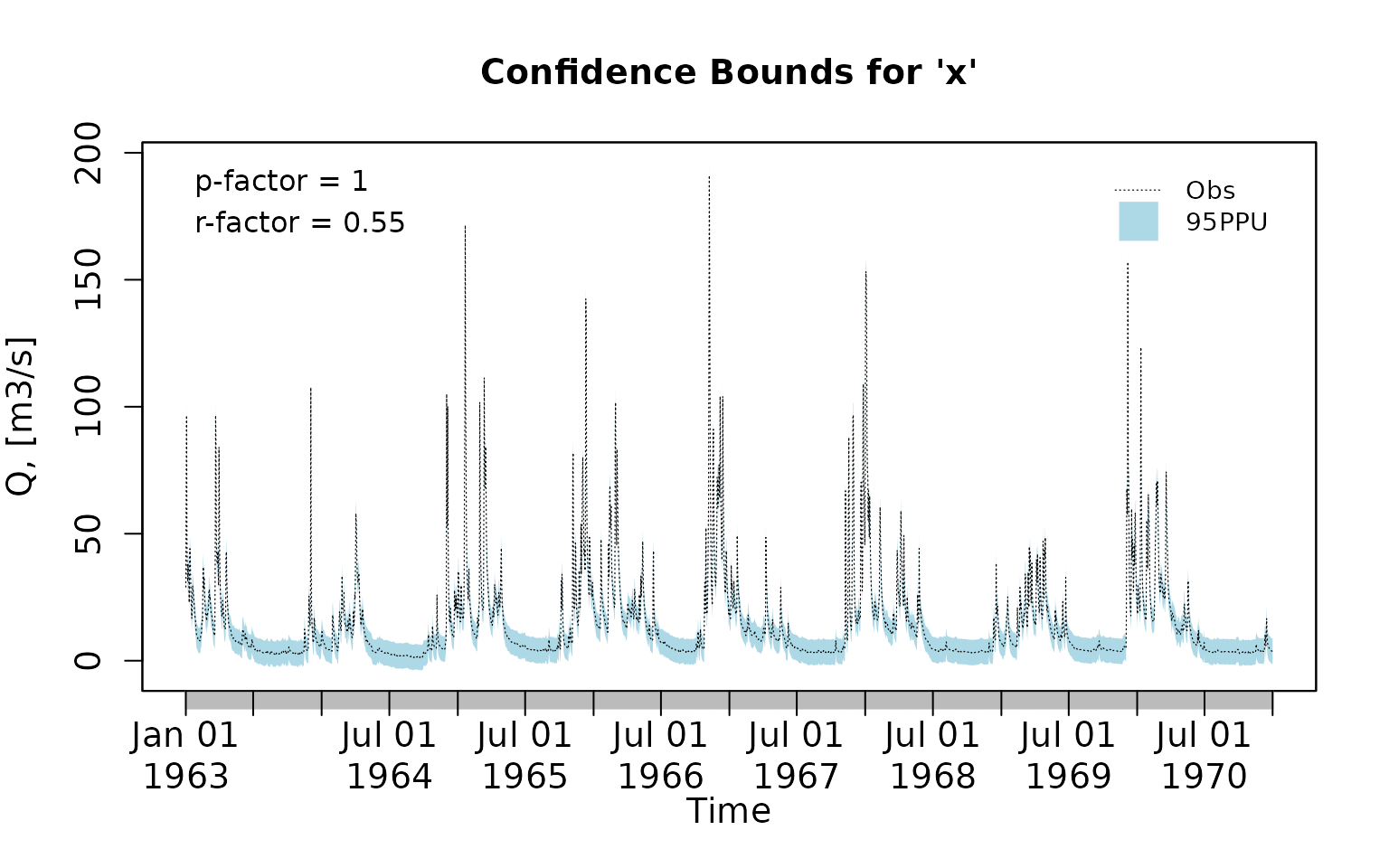

Randomly generating a simulated time series:

sim <- obs + rnorm(length(obs), mean=3)

Plotting the previously generated simulated time series along the observations and the uncertainty bounds:

plotbands(obs, lband, uband, sim)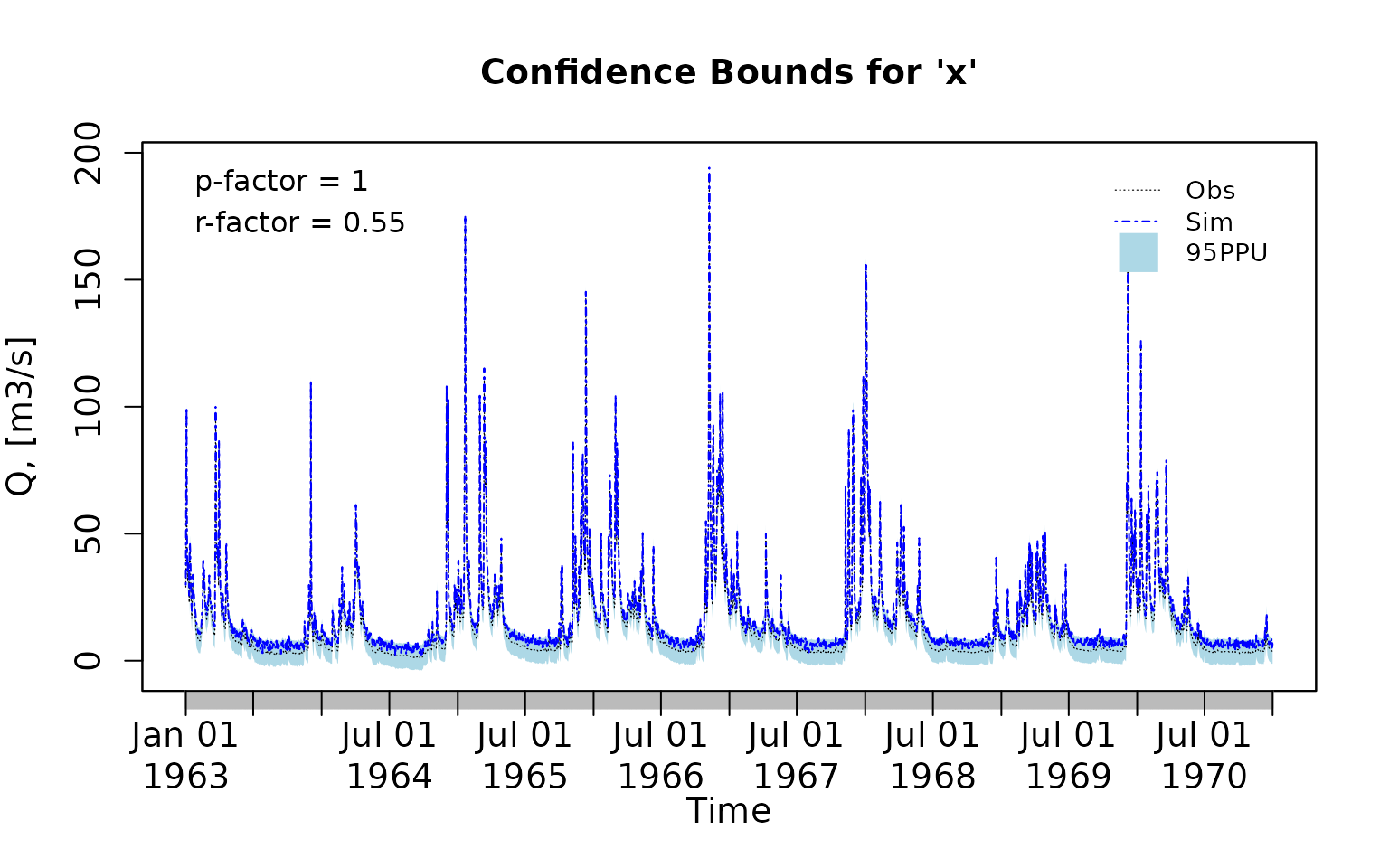

Computing P-factor

The P-factor quantifies the percentage of observed values that fall within the prediction uncertainty band defined by the lower and upper bounds. It is a measure of the coverage of the uncertainty interval.

The P-factor ranges from 0 to 1. A value of 1 indicates that all observations are bracketed by the uncertainty bounds, whereas a value of 0 indicates that none of the observations fall within the bounds.

Computing the P-factor:

( pfactor(x=obs, lband=lband, uband=uband) )

## [1] 0.9993155

Computing R-factor

The R-factor quantifies the average width of the prediction uncertainty band relative to the variability of the observed data. It is a measure of the magnitude of predictive uncertainty associated with a model simulation.

The R-factor ranges from 0 to infinity, with an optimal value of 0 indicating perfect agreement between simulated and observed values (i.e., zero prediction uncertainty). In practical applications, the R-factor represents the width of the uncertainty interval and should be as small as possible. Values close to or smaller than 1 are commonly considered indicative of an acceptable level of predictive uncertainty, although acceptable thresholds depend on the quality of observations and the modelling context.

Computing the R-factor:

( rfactor(x=obs, lband=lband, uband=uband) )

## [1] 0.5488274

Important note:

Because a larger fraction of observations can often be bracketed by widening the uncertainty bounds, the R-factor is typically interpreted jointly with the P-factor. A balance between a high P-factor (good coverage) and a low R-factor (narrow uncertainty bounds) is therefore sought during model calibration and uncertainty analysis.

Analysis of the residuals

Computing the daily residuals (even if this is a dummy example, it is enough for illustrating the capability)

r <- sim-obs

Summarizing and plotting the residuals (it requires the hydroTSM package):

library(hydroTSM)
smry(r)

##               Index         r
## Min.     1963-01-01   -0.3042
## 1st Qu.  1964-12-31    2.3620
## Median   1966-12-31    3.0400
## Mean     1966-12-31    3.0310
## 3rd Qu.  1968-12-30    3.7110
## Max.     1970-12-31    6.4810
## IQR            <NA>    1.3488
## sd             <NA>    1.0070
## cv             <NA>    0.3323
## Skewness       <NA>   -0.0700
## Kurtosis       <NA>   -0.0253
## NA's           <NA>    2.0000
## n              <NA> 2922.0000

# daily, monthly and annual plots, boxplots and histograms
hydroplot(r, FUN=mean)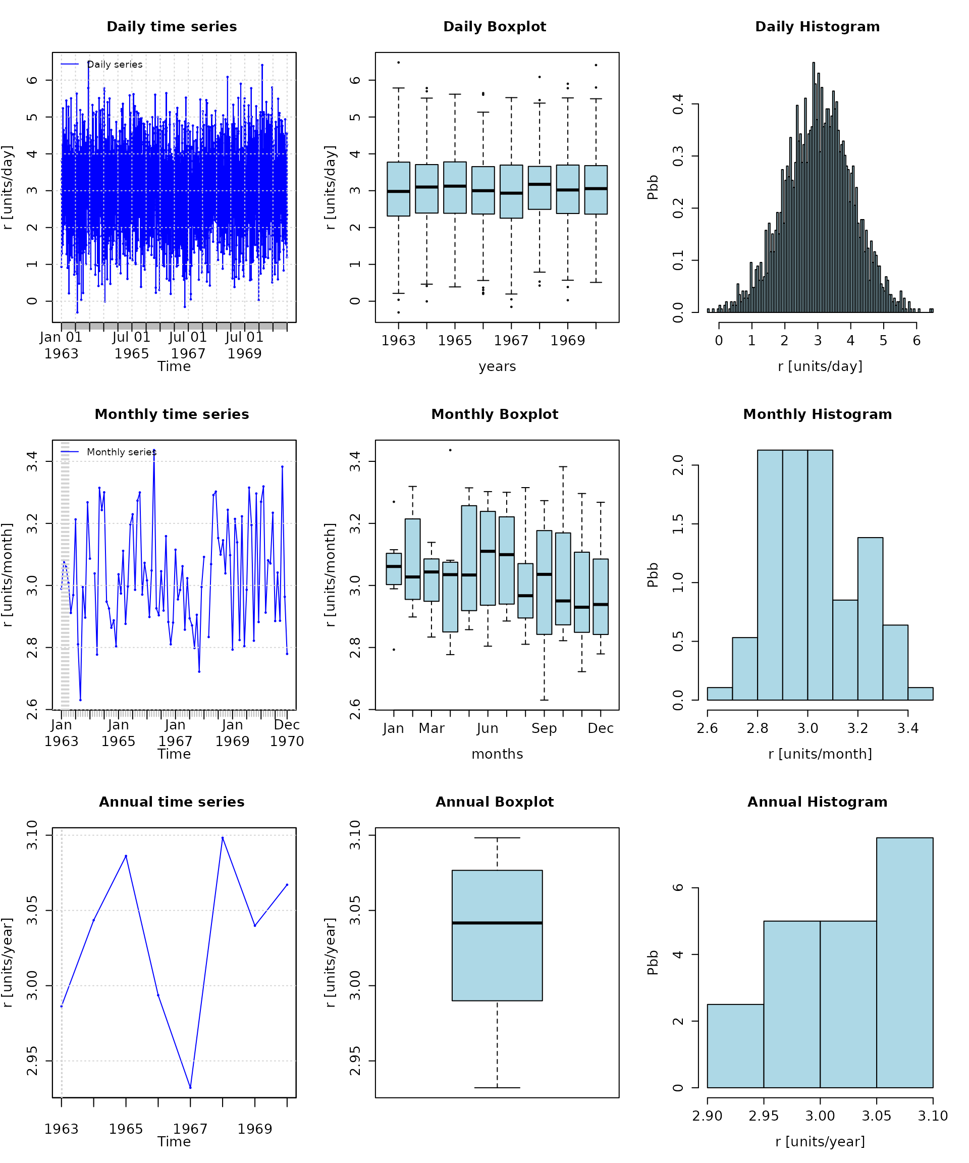

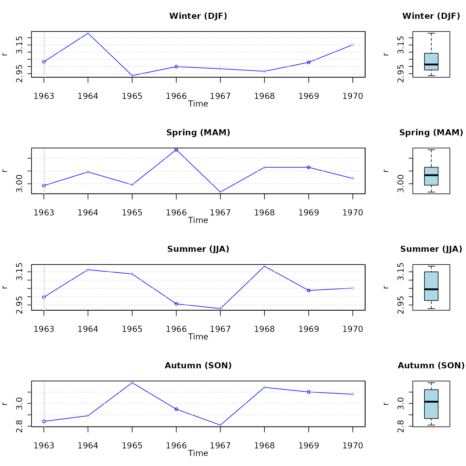
Seasonal plots and boxplots

# daily, monthly and annual plots, boxplots and histograms
hydroplot(r, FUN=mean, pfreq="seasonal")

Software details

This tutorial was built under:

## [1] "x86_64-pc-linux-gnu"

## [1] "R version 4.6.0 (2026-04-24)"

## [1] "hydroGOF 0.7-0"

Version history of this vignette

v0.4: 30-Apr-2026
v0.3: 21-Jan-2024
v0.2: Mar-2020
v0.1: Aug 2011

Mauricio Zambrano-Bigiarini¹

version 0.4, 30-Apr-2026

Citation

Installation

Setting up the environment

Example using NSE

Ex 1: ideal integer values

Ex 2: ideal real values

Ex 3: ideal daily ts

Ex 4: random noise in the first half of the simulated values

Ex 5: random noise and logarithmic transformation

Ex 6: random noise, logarithmic transformation and Pushpalatha2012 constant

Ex 7: random noise, logarithmic transformation and user-defined constant

Ex 8: random noise, logarithmic transformation and user-defined factor

Ex 9: random noise, user-defined transformation

A short example from hydrological modelling

Removing warm-up period

Plotting uncertainty bands

Computing P-factor

Computing R-factor

Analysis of the residuals

Software details

Version history of this vignette

Goodness-of-fit measures to compare observed and simulated time series with hydroGOF

Mauricio Zambrano-Bigiarini1

version 0.4, 30-Apr-2026

Citation

Installation

Setting up the environment

Example using NSE

Ex 1: ideal integer values

Ex 2: ideal real values

Ex 3: ideal daily ts

Ex 4: random noise in the first half of the simulated values

Ex 5: random noise and logarithmic transformation

Ex 6: random noise, logarithmic transformation and Pushpalatha2012 constant

Ex 7: random noise, logarithmic transformation and user-defined constant

Ex 8: random noise, logarithmic transformation and user-defined factor

Ex 9: random noise, user-defined transformation

A short example from hydrological modelling

Removing warm-up period

Plotting uncertainty bands

Computing P-factor

Computing R-factor

Analysis of the residuals

Software details

Version history of this vignette

Mauricio Zambrano-Bigiarini¹