Joint Divergence Kling-Gupta Efficiency

Joint Divergence Kling-Gupta Efficiency between sim and obs, with treatment of missing values.

This implementation follows the technical formulation described by Ficchi et al. (2026), using by defualt the KGE-2012 variability term, and computing the distributional component from a histogram-based Jensen-Shannon divergence applied to log-transformed flows after paper-specific zero handling. However, this function also allows JDKGE-style variants based on the 2009 and 2021 KGE formulations, different methods for the distributional component, and different methods for the handling of low streamflow values.

Results by Ficchi et al. (2026) show that calibrations using JDKGE significantly improve low-flow simulations compared to KGE, NSE and other competitors, while maintaining comparable or improved performance in other regimes, including high flows.

Usage

JDKGE(sim, obs, ...)

# Default S3 method
JDKGE(sim, obs, na.rm=TRUE, s=c(1,1,1,1),
        method=c("2012", "2009", "2021"), out.type=c("single", "full"), 
        density.method=c("hist", "kde", "wasserstein"), nbins="paper",
        timestep=86400, kde.n.grid=512, wasserstein.n.quantiles=512, fun=NULL, ...,
        epsilon.type=c("otherValue", "none", "Pushpalatha2012", "otherFactor"),
        epsilon.value=NA)

# S3 method for class 'data.frame'
JDKGE(sim, obs, na.rm=TRUE, s=c(1,1,1,1),
        method=c("2012", "2009", "2021"), out.type=c("single", "full"), 
        density.method=c("hist", "kde", "wasserstein"), nbins="paper",
        timestep=86400, kde.n.grid=512, wasserstein.n.quantiles=512, fun=NULL, ...,
        epsilon.type=c("otherValue", "none", "Pushpalatha2012", "otherFactor"),
        epsilon.value=NA)

# S3 method for class 'matrix'
JDKGE(sim, obs, na.rm=TRUE, s=c(1,1,1,1),
        method=c("2012", "2009", "2021"), out.type=c("single", "full"), 
        density.method=c("hist", "kde", "wasserstein"), nbins="paper",
        timestep=86400, kde.n.grid=512, wasserstein.n.quantiles=512, fun=NULL, ...,
        epsilon.type=c("otherValue", "none", "Pushpalatha2012", "otherFactor"),
        epsilon.value=NA)

# S3 method for class 'zoo'
JDKGE(sim, obs, na.rm=TRUE, s=c(1,1,1,1),
        method=c("2012", "2009", "2021"), out.type=c("single", "full"), 
        density.method=c("hist", "kde", "wasserstein"), nbins="paper",
        timestep=86400, kde.n.grid=512, wasserstein.n.quantiles=512, fun=NULL, ...,
        epsilon.type=c("otherValue", "none", "Pushpalatha2012", "otherFactor"),
        epsilon.value=NA)

Arguments

sim: numeric, zoo, matrix or data.frame with simulated values.
obs: numeric, zoo, matrix or data.frame with observed values.
na.rm: logical value indicating whether missing paired values should be removed before computing the metric.
s: numeric of length 4 with scaling factors for the Euclidean distance in criteria space. If s differs from c(1,1,1,1), then sum(s) must be equal to 1.
method: character string indicating the Kling-Gupta formulation used by JDKGE. Valid values are "2012" (default, the paper's KGE' formulation), "2009", and "2021".
out.type: character string indicating the output format. Use "single" to return the JDKGE value only, or "full" to also return the four diagnostic components.
density.method: character, representing the method used to compute the divergence component. "hist" uses the paper-faithful histogram-based Jensen-Shannon divergence, "kde" uses a common-grid kernel density estimate followed by Jensen-Shannon divergence, and "wasserstein" uses a Wasserstein-distance similarity on log-flows.
nbins: character, representing the binning rule used by the histogram divergence component. The default "paper" uses the procedure described by Ficchi et al. (2026). This argument is ignored for density.method="kde" and density.method="wasserstein".
timestep: numeric, representing the sampling time step in seconds used by the paper's bin-count adjustment. For zoo inputs this is inferred from the time index when omitted. The default for plain numeric vectors is one day (86400 seconds).
kde.n.grid: integer, number of grid points used when density.method="kde". Larger values provide a finer common support grid at higher computational cost.
wasserstein.n.quantiles: integer, number of quantile levels used to approximate the first Wasserstein distance when density.method="wasserstein". Larger values provide a finer approximation at higher computational cost.
fun: optional function applied to sim and obs before computing JDKGE. The first argument of fun must be a numeric vector.
...: additional arguments passed to fun.
epsilon.type: rule used for zero-flow handling in the internal log-based divergence component, and also passed to preproc when fun needs an offset before transformation. The default is "otherValue".
epsilon.value: numeric value used when epsilon.type="otherValue" or epsilon.type="otherFactor". When epsilon.type="otherValue" and epsilon.value=NA (the default), the value described by Ficchi et al. (2026), $\epsilon = \min(10^{-6}, 10^{-1} \min(c))$, is computed internally.

Details

JDKGE combines four components:

the Pearson correlation coefficient $r$,
the variability term, defined as $\gamma = (\sigma_s / \mu_s) / (\sigma_o / \mu_o)$ for method="2012" and as $\alpha = \sigma_s / \sigma_o$ for method="2009" and method="2021",
the bias term, defined as $\beta = \mu_s / \mu_o$ for method="2009" and method="2012", and as $\beta_{2021} = (\mu_s - \mu_o)/\sigma_o$ for method="2021", and
the distributional similarity component $\Delta$.

For the divergence component, this implementation follows the paper's workflow:

exact zeros are replaced according to epsilon.type. With the default "otherValue" and epsilon.value=NA, $\epsilon = \min(10^{-6}, 10^{-1} \min(c))$, where $c$ is the set of strictly positive simulated and observed values,
the transformed values $\log(x)$ are binned using a histogram,
the Freedman-Diaconis width is lower-bounded by $h_{min} = \min(10^2 \epsilon, 10^{-1})$,
the number of bins is adjusted by the time-scale factor and clipped to the interval $[25, 100]$,
additive smoothing with $\alpha = \epsilon$ is applied to the empirical densities, and
Jensen-Shannon divergence is computed with base-2 logarithms.

For density.method="kde", simulated and observed log-flows are smoothed with Gaussian kernel density estimates evaluated on a common grid over the pooled support using a shared bandwidth estimated from the pooled sample. Jensen-Shannon divergence is then computed from the two resulting probability vectors.

For density.method="wasserstein", the log-flow distributions are compared with the first Wasserstein distance computed from empirical quantiles. The resulting distance is converted into a similarity component through $$\Delta = \exp(-W_1 / s_w)$$ where $s_w$ is a robust scale estimated from the pooled log-flows using the interquartile range, with fallback to the standard deviation when needed.

The metric is then computed as:

$$JDKGE = 1 - \sqrt{(s[1](r-1))^2 + (s[2](vr-1))^2 + (s[3](br-1))^2 + (s[4](\Delta-1))^2}$$

Joint Divergence Kling-Gupta efficiencies range from $-\infty$ to 1. Values closer to 1 indicate stronger agreement between simulated and observed values across correlation, variability, bias, and distributional similarity.

Value

If out.type="single": numeric with the Joint Divergence Kling-Gupta Efficiency between sim and obs. If sim and obs are matrices, the output is a vector with one efficiency value per column pair.

If out.type="full": a list with two elements:

JDKGE.value: numeric with the Joint Divergence Kling-Gupta Efficiency.
JDKGE.elements: numeric with 4 elements: ‘r’, the selected bias term, the selected variability term, and ‘Delta’.

References

Ficchi, A.; Bavera, D.; Grimaldi, S.; Moschini, F.; Pistocchi, A.; Russo, C.; Salamon, P.; Toreti, A. (2026). Improving low and high flow simulations at once: An enhanced metric for hydrological model calibrations. EGUsphere [preprint], https://doi.org/10.5194/egusphere-2026-43.

Kling, H.; Fuchs, M.; Paulin, M. (2012). Runoff conditions in the upper Danube basin under an ensemble of climate change scenarios. Journal of Hydrology, 424, 264-277, doi:10.1016/j.jhydrol.2012.01.011.

Tang, G.; Clark, M.P.; Papalexiou, S.M. (2021). SC-earth: a station-based serially complete earth dataset from 1950 to 2019. Journal of Climate, 34(16), 6493-6511. doi:10.1175/JCLI-D-21-0067.1.

Examples

# Example 0.1: ideal case
obs <- 1:10
sim <- 1:10

JDKGE(sim, obs)
#> [1] 1

##################
# Example 1: simulated values equal to twice the observations
sim <- 2*obs
JDKGE(sim=sim, obs=obs, out.type="full")
#> $JDKGE.value
#> [1] -0.1180287
#> 
#> $JDKGE.elements
#>         r      Beta     Gamma     Delta 
#> 1.0000000 2.0000000 1.0000000 0.5000119 
#> 

##################
# Example 2: using kernel density estimation, instead of histograms (the default)
JDKGE(sim=sim, obs=obs, density.method="kde")
#> [1] -0.005512615
JDKGE(sim=sim, obs=obs, density.method="kde", kde.n.grid=1024)
#> [1] -0.005471278
JDKGE(sim=sim, obs=obs, density.method="wasserstein")
#> [1] -0.1241596
JDKGE(sim=sim, obs=obs, density.method="wasserstein", wasserstein.n.quantiles=1024)
#> [1] -0.1241596

##################
# Example 3: Looking at the difference between JDKGE and KGE, both with 'method=2009' 
#            and 'method=2012'
# Loading daily streamflows of the Ega River (Spain), from 1961 to 1970
data(EgaEnEstellaQts)
obs <- EgaEnEstellaQts

# Simulated daily time series, initially equal to twice the observed values
sim <- 2*obs 

# KGE 2009
KGE(sim=sim, obs=obs, method="2009", out.type="full")
#> $KGE.value
#> [1] -0.4142136
#> 
#> $KGE.elements
#>     r  Beta Alpha 
#>     1     2     2 
#> 

# JDKGE (Ficchi et al., 2026):
JDKGE(sim=sim, obs=obs, method="2009", out.type="full")
#> $JDKGE.value
#> [1] -0.4243983
#> 
#> $JDKGE.elements
#>         r      Beta     Alpha     Delta 
#> 1.0000000 2.0000000 2.0000000 0.8299693 
#> 

# KGE 2012
KGE(sim=sim, obs=obs, method="2012", out.type="full")
#> $KGE.value
#> [1] 0
#> 
#> $KGE.elements
#>     r  Beta Gamma 
#>     1     2     1 
#> 

# JDKGE (Ficchi et al., 2026):
JDKGE(sim=sim, obs=obs, method="2012", out.type="full")
#> $JDKGE.value
#> [1] -0.01435222
#> 
#> $JDKGE.elements
#>         r      Beta     Gamma     Delta 
#> 1.0000000 2.0000000 1.0000000 0.8299693 
#> 

# KGE 2021
KGE(sim=sim, obs=obs, method="2021", out.type="full")
#> $KGE.value
#> [1] -0.2744084
#> 
#> $KGE.elements
#>         r Beta.2021     Alpha 
#> 1.0000000 0.7900105 2.0000000 
#> 

# JDKGE (Ficchi et al., 2026):
JDKGE(sim=sim, obs=obs, method="2021", out.type="full")
#> $JDKGE.value
#> [1] -0.03586003
#> 
#> $JDKGE.elements
#>         r Beta.2021     Alpha     Delta 
#> 1.0000000 0.7900105 2.0000000 0.8299693 
#> 

##################
# Example 4: 
# Loading daily streamflows of the Ega River (Spain), from 1961 to 1970
data(EgaEnEstellaQts)
obs <- EgaEnEstellaQts

# Generating a simulated daily time series, initially equal to the observed series
sim <- obs 

# Computing the 'JDKGE' for the "best" (unattainable) case
JDKGE(sim=sim, obs=obs)
#> [1] 1

##################
# Example 5: JDKGE for simulated values equal to observations plus random noise 
#            on the first half of the observed values. 
#            This random noise has more relative importance for ow flows than 
#            for medium and high flows.
  
# Randomly changing the first 1826 elements of 'sim', by using a normal distribution 
# with mean 10 and standard deviation equal to 1 (default of 'rnorm').
sim[1:1826] <- obs[1:1826] + rnorm(1826, mean=10)
ggof(sim, obs)


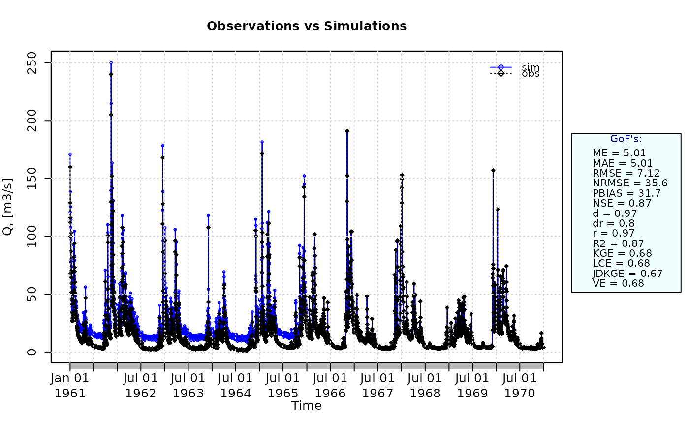JDKGE(sim=sim, obs=obs)
#> [1] 0.6083153

##################
# Example 6: JDKGE for simulated values equal to observations plus random noise 
#            on the first half of the observed values and applying a 
#            user-defined function to 'sim' and 'obs' during computations

fun1 <- function(x) {sqrt(x+1)}

JDKGE(sim=sim, obs=obs, fun=fun1)
#> [1] 0.7286612

# Verifying the previous value
sim1 <- sqrt(sim+1)
obs1 <- sqrt(obs+1)
JDKGE(sim=sim1, obs=obs1)
#> [1] 0.7286612

##################
# Example 7: JDKGE for a two-column data frame where simulated values are equal to 
#            observations plus random noise on the first half of the observed values 

SIM <- cbind(sim, sim)
OBS <- cbind(obs, obs)

JDKGE(sim=SIM, obs=OBS)
#>       obs       obs 
#> 0.6083153 0.6083153