Median annual high-flow bias

Median annual high-flow bias between sim and obs, with treatment of missing values and explicit focus on the reproduction of high-flow events.

This function is designed to identify differences in high values. See Details.

Usage

HFB(sim, obs, ...)

# Default S3 method
HFB(sim, obs, na.rm=TRUE, 
             hQ.thr=0.1, start.month=1, out.PerYear=FALSE,
             fun=NULL, ...,
             epsilon.type=c("none", "Pushpalatha2012", "otherFactor", "otherValue"), 
             epsilon.value=NA)

# S3 method for class 'data.frame'
HFB(sim, obs, na.rm=TRUE, 
             hQ.thr=0.1, start.month=1, out.PerYear=FALSE,
             fun=NULL, ...,
             epsilon.type=c("none", "Pushpalatha2012", "otherFactor", "otherValue"), 
             epsilon.value=NA)

# S3 method for class 'matrix'
HFB(sim, obs, na.rm=TRUE, 
             hQ.thr=0.1, start.month=1, out.PerYear=FALSE,
             fun=NULL, ...,
             epsilon.type=c("none", "Pushpalatha2012", "otherFactor", "otherValue"), 
             epsilon.value=NA)
             
# S3 method for class 'zoo'
HFB(sim, obs, na.rm=TRUE, 
             hQ.thr=0.1, start.month=1, out.PerYear=FALSE,
             fun=NULL, ...,
             epsilon.type=c("none", "Pushpalatha2012", "otherFactor", "otherValue"), 
             epsilon.value=NA)

Arguments

sim

numeric, zoo, matrix or data.frame with simulated values

obs

numeric, zoo, matrix or data.frame with observed values

na.rm

a logical value indicating whether 'NA' should be stripped before the computation proceeds.
When an 'NA' value is found at the i-th position in obs OR sim, the i-th value of obs AND sim are removed before the computation.

hQ.thr

numeric, representing the exceedence probabiliy used to identify high flows in obs. All values in obs that are equal or higher than quantile(obs, probs=(1-hQ.thr)) are considered as high flows. By default hQ.thr=0.1.
On the other hand, the high values in sim are those located at the same i-th position than the i-th value of the obs deemed as high flows.

start.month

[OPTIONAL]. Only used when the (hydrological) year of interest is different from the calendar year.

numeric in [1:12] indicating the starting month of the (hydrological) year. Numeric values in [1, 12] represent months in [January, December]. By default start.month=1.

out.PerYear

logical, indicating whether the output of this function has to include the median annual high-flows bias obtained for the individual years in sim and obs or not.

fun

function to be applied to sim and obs in order to obtain transformed values thereof before computing this goodness-of-fit index.

The first argument MUST BE a numeric vector with any name (e.g., x), and additional arguments are passed using ....

...

arguments passed to fun, in addition to the mandatory first numeric vector.

epsilon.type

argument used to define a numeric value to be added to both sim and obs before applying fun.

It is was designed to allow the use of logarithm and other similar functions that do not work with zero values.

Valid values of epsilon.type are:

1) "none": sim and obs are used by fun without the addition of any numeric value. This is the default option.

2) "Pushpalatha2012": one hundredth (1/100) of the mean observed values is added to both sim and obs before applying fun, as described in Pushpalatha et al. (2012).

3) "otherFactor": the numeric value defined in the epsilon.value argument is used to multiply the the mean observed values, instead of the one hundredth (1/100) described in Pushpalatha et al. (2012). The resulting value is then added to both sim and obs, before applying fun.

4) "otherValue": the numeric value defined in the epsilon.value argument is directly added to both sim and obs, before applying fun.

epsilon.value

-) when epsilon.type="otherValue" it represents the numeric value to be added to both sim and obs before applying fun.

-) when epsilon.type="otherFactor" it represents the numeric factor used to multiply the mean of the observed values, instead of the one hundredth (1/100) described in Pushpalatha et al. (2012). The resulting value is then added to both sim and obs before applying fun.

Details

The median annual high-flow bias (HFB) is a goodness-of-fit metric designed to support the calibration and evaluation of hydrological models with specific emphasis on the reproduction of high-flow conditions.

The HFB ranges from 0 to Inf, with an optimal value of 0. Values close to 0 indicate that the simulated high flows closely match the observed high flows, whereas larger values indicate increasing discrepancies between the simulated and observed high-flow magnitudes.

The current formulation of the HFB function was proposed by Zambrano-Bigiarini (2026), inspired by the annual peak-flow bias (APFB) objective function proposed by Mizukami et al. (2019). However, HFB differs from APFB in four important aspects:

1) Instead of considering only the single observed annual peak flow in each year, it considers all high flows in each year, where "high flows" are defined as all values equal to or greater than a user-defined exceedance probability threshold of the observed values. By default, high flows correspond to the upper 10% of observed flows (i.e., hQ.thr=0.1).

2) Instead of selecting simulated high flows independently of the observed events, it evaluates simulated flows occurring at the same time steps as the observed high flows, thereby preserving temporal correspondence between observed and simulated events.

3) For each year, the metric uses the median of the individual high-flow ratios rather than a single annual peak-flow value, providing a more robust summary of high-flow bias within that year.

4) When computing the final performance value, the metric uses the median of the annual values instead of the mean, reducing the influence of extreme years and improving robustness when the distribution of annual biases is asymmetric.

Mathematically, the annual high-flow bias for year $y$ is defined as:

$$ HFB_y = \sqrt{\left(\frac{\operatorname{median}(Q^{sim}_{y,i})}{\operatorname{median}(Q^{obs}_{y,i})} - 1\right)^2} $$

where $Q^{sim}_{y,i}$ and $Q^{obs}_{y,i}$ are the simulated and observed flows corresponding to the set of high-flow events $i$ occurring in year $y$.

The overall HFB value is then computed as:

$$ HFB = \operatorname{median}(HFB_y) $$

This formulation yields a non-negative bias metric, with the minimum value of 0 representing perfect agreement between simulated and observed high flows.

Value

If out.PerYear=FALSE: numeric with the median annual high-flow bias between sim and obs. If sim and obs are matrices, the output value is a vector, with the high-flow bias between each column of sim and obs.

If out.PerYear=TRUE: a list of two elements:

HFB.value

numeric with the median annual high flow bias between sim and obs. If sim and obs are matrices, the output value is a vector, with the median annual high flow bias between each column of sim and obs.

HFB.PerYear

-) If sim and obs are not data.frame/matrix, the output is numeric, with the median high flow bias obtained for the individual years between sim and obs.

-) If sim and obs are data.frame/matrix, this output is a data.frame, with the median high flow bias obtained for the individual years between sim and obs.

References

Zambrano-Bigiarini, Mauricio (2026). hydroGOF: Goodness-of-fit functions for comparison of simulated and observed hydrological time series. R package version 0.7-0. URL:https://cran.r-project.org/package=hydroGOF. doi:10.32614/CRAN.package.hydroGOF.

Mizukami, N.; Rakovec, O.; Newman, A.J.; Clark, M.P.; Wood, A.W.; Gupta, H.V.; Kumar, R.: (2019). On the choice of calibration metrics for "high-flow" estimation using hydrologic models, Hydrology Earth System Sciences 23, 2601-2614, doi:10.5194/hess-23-2601-2019.

Author

Mauricio Zambrano-Bigiarini <mzb.devel@gmail.com>

Note

obs and sim has to have the same length/dimension

The missing values in obs and sim are removed before the computation proceeds, and only those positions with non-missing values in obs and sim are considered in the computation

Examples

##################
# Example 1: Looking at the difference between 'NSE', 'wNSE', and 'HFB'
# Loading daily streamflows of the Ega River (Spain), from 1961 to 1970
data(EgaEnEstellaQts)
obs <- EgaEnEstellaQts

# Simulated daily time series, created equal to the observed values and then 
# random noise is added only to high flows, i.e., those equal or higher than 
# the quantile 0.9 of the observed values.
sim      <- obs
hQ.thr   <- quantile(obs, probs=0.9, na.rm=TRUE)
hQ.index <- which(obs >= hQ.thr)
hQ.n     <- length(hQ.index)
sim[hQ.index] <- sim[hQ.index] + rnorm(hQ.n, mean=mean(sim[hQ.index], na.rm=TRUE))

# Traditional Nash-Sutcliffe eficiency
NSE(sim=sim, obs=obs)
#> [1] 0.005488789

# Weighted Nash-Sutcliffe efficiency (Hundecha and Bardossy, 2004)
wNSE(sim=sim, obs=obs)
#> [1] 0.2825219

# HFB (Garcia et al., 2017):
HFB(sim=sim, obs=obs)
#> [1] 1.149116

##################
# Example 2: 
# Loading daily streamflows of the Ega River (Spain), from 1961 to 1970
data(EgaEnEstellaQts)
obs <- EgaEnEstellaQts

# Generating a simulated daily time series, initially equal to the observed series
sim <- obs 

# Computing the 'HFB' for the "best" (unattainable) case
HFB(sim=sim, obs=obs)
#> [1] 0

##################
# Example 3: HFB for simulated values created equal to the observed values and then 
#            random noise is added only to high flows, i.e., those equal or higher than 
#            the quantile 0.9 of the observed values.

sim           <- obs
hQ.thr        <- quantile(obs, hQ.thr=0.9, na.rm=TRUE)
hQ.index      <- which(obs >= hQ.thr)
#> Warning: longer object length is not a multiple of shorter object length
hQ.n          <- length(hQ.index)
sim[hQ.index] <- sim[hQ.index] + rnorm(hQ.n, mean=mean(sim[hQ.index], na.rm=TRUE))
ggof(sim, obs)


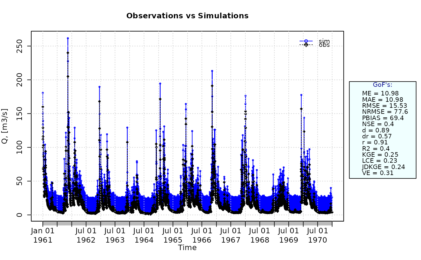HFB(sim=sim, obs=obs)
#> [1] 0.3506699

##################
# Example 4: HFB for simulated values created equal to the observed values and then 
#            random noise is added only to high flows, i.e., those equal or higher than 
#            the quantile 0.9 of the observed values and applying (natural) 
#            logarithm to 'sim' and 'obs' during computations.

HFB(sim=sim, obs=obs, fun=log)
#> [1] 0.07488176

# Verifying the previous value:
lsim <- log(sim)
lobs <- log(obs)
HFB(sim=lsim, obs=lobs)
#> [1] 0.07488176


##################
# Example 5: HFB for simulated values created equal to the observed values and then 
#            random noise is added only to high flows, i.e., those equal or higher than 
#            the quantile 0.9 of the observed values and applying a 
#            user-defined function to 'sim' and 'obs' during computations

fun1 <- function(x) {sqrt(x+1)}

HFB(sim=sim, obs=obs, fun=fun1)
#> [1] 0.1594608

# Verifying the previous value
sim1 <- sqrt(sim+1)
obs1 <- sqrt(obs+1)
HFB(sim=sim1, obs=obs1)
#> [1] 0.1594608