Percent Bias

Percent Bias between sim and obs, with treatment of missing values.

Usage

pbias(sim, obs, ...)

# Default S3 method
pbias(sim, obs, na.rm=TRUE, dec=1, fun=NULL, ..., 
               epsilon.type=c("none", "Pushpalatha2012", "otherFactor", "otherValue"), 
               epsilon.value=NA)

# S3 method for class 'data.frame'
pbias(sim, obs, na.rm=TRUE, dec=1, fun=NULL, ..., 
               epsilon.type=c("none", "Pushpalatha2012", "otherFactor", "otherValue"), 
               epsilon.value=NA)

# S3 method for class 'matrix'
pbias(sim, obs, na.rm=TRUE, dec=1, fun=NULL, ..., 
               epsilon.type=c("none", "Pushpalatha2012", "otherFactor", "otherValue"), 
               epsilon.value=NA)

# S3 method for class 'zoo'
pbias(sim, obs, na.rm=TRUE, dec=1, fun=NULL, ..., 
               epsilon.type=c("none", "Pushpalatha2012", "otherFactor", "otherValue"), 
               epsilon.value=NA)

Arguments

sim

numeric, zoo, matrix or data.frame with simulated values

obs

numeric, zoo, matrix or data.frame with observed values

na.rm

a logical value indicating whether 'NA' should be stripped before the computation proceeds.
When an 'NA' value is found at the i-th position in obs OR sim, the i-th value of obs AND sim are removed before the computation.

dec

numeric, specifying the number of decimal places used to rounf the output object. Default value is 1.

fun

function to be applied to sim and obs in order to obtain transformed values thereof before computing this goodness-of-fit index.

The first argument MUST BE a numeric vector with any name (e.g., x), and additional arguments are passed using ....

...

arguments passed to fun, in addition to the mandatory first numeric vector.

epsilon.type

argument used to define a numeric value to be added to both sim and obs before applying fun.

It is was designed to allow the use of logarithm and other similar functions that do not work with zero values.

Valid values of epsilon.type are:

1) "none": sim and obs are used by fun without the addition of any numeric value. This is the default option.

2) "Pushpalatha2012": one hundredth (1/100) of the mean observed values is added to both sim and obs before applying fun, as described in Pushpalatha et al. (2012).

3) "otherFactor": the numeric value defined in the epsilon.value argument is used to multiply the the mean observed values, instead of the one hundredth (1/100) described in Pushpalatha et al. (2012). The resulting value is then added to both sim and obs, before applying fun.

4) "otherValue": the numeric value defined in the epsilon.value argument is directly added to both sim and obs, before applying fun.

epsilon.value

-) when epsilon.type="otherValue" it represents the numeric value to be added to both sim and obs before applying fun.
-) when epsilon.type="otherFactor" it represents the numeric factor used to multiply the mean of the observed values, instead of the one hundredth (1/100) described in Pushpalatha et al. (2012). The resulting value is then added to both sim and obs before applying fun.

Details

$$PBIAS = 100 \frac{ \sum_{i=1}^N { \left( S_i - O_i \right) } } { \sum_{i=1}^N O_i} $$

Percent bias (PBIAS) measures the average tendency of the simulated values to be larger or smaller than their observed ones.

The optimal value of PBIAS is 0.0, with low-magnitude values indicating accurate model simulation. Positive values indicate overestimation bias, whereas negative values indicate model underestimation bias

Value

Percent bias between sim and obs. The result is given in percentage (%)

If sim and obs are matrixes, the returned value is a vector, with the percent bias between each column of sim and obs.

References

Yapo, P.O.; Gupta, H.V.; Sorooshian S. (1996). Automatic calibration of conceptual rainfall-runoff models: sensitivity to calibration data. Journal of Hydrology. v181 i1-4. 23–48. doi:10.1016/0022-1694(95)02918-4

Sorooshian, S., Q. Duan, and V. K. Gupta. 1993. Calibration of rainfall-runoff models: Application of global optimization to the Sacramento Soil Moisture Accounting Model, Water Resources Research, 29 (4), 1185-1194, doi:10.1029/92WR02617.

Author

Mauricio Zambrano Bigiarini <mzb.devel@gmail.com>

Note

obs and sim has to have the same length/dimension

The missing values in obs and sim are removed before the computation proceeds, and only those positions with non-missing values in obs and sim are considered in the computation

Examples

##################
# Example 1: basic ideal case
obs <- 1:10
sim <- 1:10
pbias(sim, obs)
#> [1] 0

obs <- 1:10
sim <- 2:11
pbias(sim, obs)
#> [1] 18.2

##################
# Example 2: 
# Loading daily streamflows of the Ega River (Spain), from 1961 to 1970
data(EgaEnEstellaQts)
obs <- EgaEnEstellaQts

# Generating a simulated daily time series, initially equal to the observed series
sim <- obs 

# Computing the 'pbias' for the "best" (unattainable) case
pbias(sim=sim, obs=obs)
#> [1] 0

##################
# Example 3: pbias for simulated values equal to observations plus random noise 
#            on the first half of the observed values. 
#            This random noise has more relative importance for ow flows than 
#            for medium and high flows.
  
# Randomly changing the first 1826 elements of 'sim', by using a normal distribution 
# with mean 10 and standard deviation equal to 1 (default of 'rnorm').
sim[1:1826] <- obs[1:1826] + rnorm(1826, mean=10)
ggof(sim, obs)


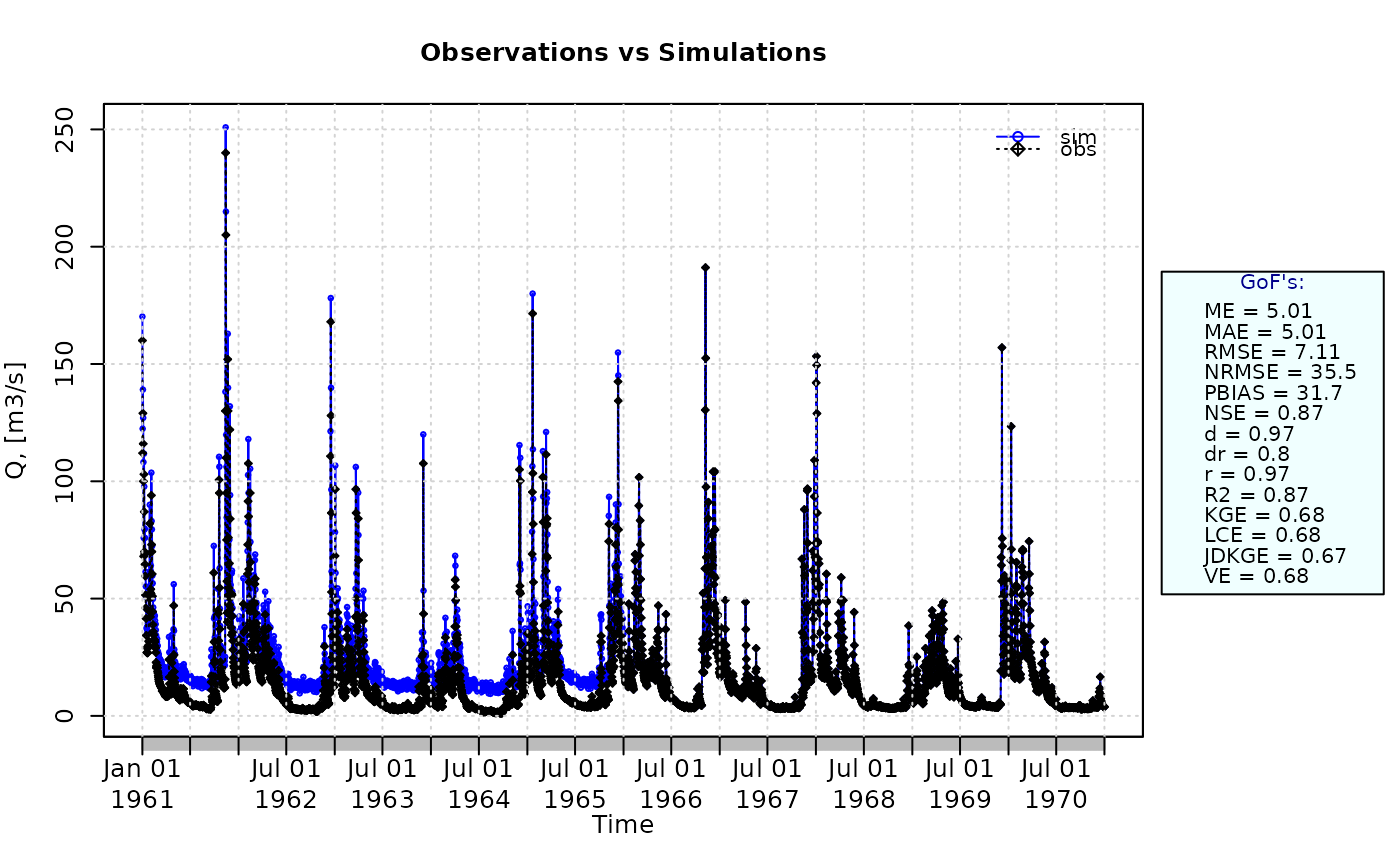pbias(sim=sim, obs=obs)
#> [1] 31.7

##################
# Example 4: pbias for simulated values equal to observations plus random noise 
#            on the first half of the observed values and applying (natural) 
#            logarithm to 'sim' and 'obs' during computations.

pbias(sim=sim, obs=obs, fun=log)
#> [1] 18.8

# Verifying the previous value:
lsim <- log(sim)
lobs <- log(obs)
pbias(sim=lsim, obs=lobs)
#> [1] 18.8

##################
# Example 5: pbias for simulated values equal to observations plus random noise 
#            on the first half of the observed values and applying (natural) 
#            logarithm to 'sim' and 'obs' and adding the Pushpalatha2012 constant
#            during computations

pbias(sim=sim, obs=obs, fun=log, epsilon.type="Pushpalatha2012")
#> [1] 18.2

# Verifying the previous value, with the epsilon value following Pushpalatha2012
eps  <- mean(obs, na.rm=TRUE)/100
lsim <- log(sim+eps)
lobs <- log(obs+eps)
pbias(sim=lsim, obs=lobs)
#> [1] 18.2

##################
# Example 6: pbias for simulated values equal to observations plus random noise 
#            on the first half of the observed values and applying (natural) 
#            logarithm to 'sim' and 'obs' and adding a user-defined constant
#            during computations

eps <- 0.01
pbias(sim=sim, obs=obs, fun=log, epsilon.type="otherValue", epsilon.value=eps)
#> [1] 18.7

# Verifying the previous value:
lsim <- log(sim+eps)
lobs <- log(obs+eps)
pbias(sim=lsim, obs=lobs)
#> [1] 18.7

##################
# Example 7: pbias for simulated values equal to observations plus random noise 
#            on the first half of the observed values and applying (natural) 
#            logarithm to 'sim' and 'obs' and using a user-defined factor
#            to multiply the mean of the observed values to obtain the constant
#            to be added to 'sim' and 'obs' during computations

fact <- 1/50
pbias(sim=sim, obs=obs, fun=log, epsilon.type="otherFactor", epsilon.value=fact)
#> [1] 17.6

# Verifying the previous value:
eps  <- fact*mean(obs, na.rm=TRUE)
lsim <- log(sim+eps)
lobs <- log(obs+eps)
pbias(sim=lsim, obs=lobs)
#> [1] 17.6

##################
# Example 8: pbias for simulated values equal to observations plus random noise 
#            on the first half of the observed values and applying a 
#            user-defined function to 'sim' and 'obs' during computations

fun1 <- function(x) {sqrt(x+1)}

pbias(sim=sim, obs=obs, fun=fun1)
#> [1] 17.7

# Verifying the previous value, with the epsilon value following Pushpalatha2012
sim1 <- sqrt(sim+1)
obs1 <- sqrt(obs+1)
pbias(sim=sim1, obs=obs1)
#> [1] 17.7