Liu-Mean Efficiency

Liu-Mean Efficiency between sim and obs, with treatment of missing values.

This goodness-of-fit measure was proposed by Liu et al. (2020) as an alternative to the Nash-Sutcliffe efficiency (NSE), designed to provide a more balanced assessment of model performance by normalising the mean squared error using the mean of the observed values instead of their variance.

The Liu-Mean Efficiency evaluates how large the error is compared to the average level of the observations, making it particularly useful in hydrological applications where the mean value is a meaningful scale for evaluating prediction accuracy.

The normalisation makes that this performance measure behave like a dimensionless relative error, scaled by the characteristic magnitude of the variable. As a result, the same absolute error will be judged differently depending on whether the mean flow is small or large.

For a short description of the metric and the numeric range of values, please see Details.

Usage

LME(sim, obs, ...)

# Default S3 method
LME(sim, obs, na.rm=TRUE, out.type=c("single","full"), fun=NULL, ...,
             epsilon.type=c("none", "Pushpalatha2012", "otherFactor", "otherValue"),
             epsilon.value=NA)

# S3 method for class 'data.frame'
LME(sim, obs, na.rm=TRUE, out.type=c("single","full"), fun=NULL, ...,
             epsilon.type=c("none", "Pushpalatha2012", "otherFactor", "otherValue"),
             epsilon.value=NA)

# S3 method for class 'matrix'
LME(sim, obs, na.rm=TRUE, out.type=c("single","full"), fun=NULL, ...,
             epsilon.type=c("none", "Pushpalatha2012", "otherFactor", "otherValue"),
             epsilon.value=NA)

# S3 method for class 'zoo'
LME(sim, obs, na.rm=TRUE, out.type=c("single","full"), fun=NULL, ...,
             epsilon.type=c("none", "Pushpalatha2012", "otherFactor", "otherValue"),
             epsilon.value=NA)

Arguments

sim

numeric, zoo, matrix or data.frame with simulated values.

obs

numeric, zoo, matrix or data.frame with observed values.

na.rm

a logical value indicating whether 'NA' should be stripped before the computation proceeds.
When an 'NA' value is found at the i-th position in obs OR sim, the i-th value of obs AND sim are removed before the computation.

out.type

character, indicating whether the output of the function has to include only the Liu-Mean Efficiency or also the intermediate quantities used in its computation. Valid values are:

-) single: the output is a numeric with the Liu-Mean Efficiency only.

-) full: the output is a list of two elements: the first one with the Liu-Mean Efficiency, and the second is a numeric with 2 elements: the mean squared error (‘MSE’) between sim and obs, and the mean of the observed values (‘MeanObs’) used as the normalization term in the computation of the Liu-Mean Efficiency.

fun

function to be applied to sim and obs in order to obtain transformed values thereof before computing the Liu-Mean Efficiency.

The first argument MUST BE a numeric vector with any name (e.g., x), and additional arguments are passed using ....

...

arguments passed to fun, in addition to the mandatory first numeric vector.

epsilon.type

argument used to define a numeric value to be added to both sim and obs before applying fun.

It is designed to allow the use of logarithm and other similar functions that do not work with zero values.

Valid values of epsilon.type are:

1) "none": sim and obs are used by fun without the addition of any numeric value.

2) "Pushpalatha2012": one hundredth (1/100) of the mean observed values is added to both sim and obs before applying fun, as described in Pushpalatha et al. (2012).

3) "otherFactor": the numeric value defined in the epsilon.value argument is used to multiply the mean observed values. The resulting value is then added to both sim and obs, before applying fun.

4) "otherValue": the numeric value defined in the epsilon.value argument is directly added to both sim and obs, before applying fun.

epsilon.value

-) when epsilon.type="otherValue" it represents the numeric value to be added to both sim and obs before applying fun.
-) when epsilon.type="otherFactor" it represents the numeric factor used to multiply the mean of the observed values. The resulting value is then added to both sim and obs before applying fun.

Details

The Liu-Mean Efficiency (LME) is based on the mean squared error (MSE) normalized by the squared mean of the observed values.

Its formulation is conceptually similar to the Nash-Sutcliffe efficiency, but uses the mean of observations as the reference scaling factor instead of the variance. This modification reduces the sensitivity of the metric to high variability and makes the performance evaluation more directly interpretable in terms of proportional error relative to the mean magnitude of the observed variable.

The Liu-Mean Efficiency ranges from -Inf to 1.

A value of:

- LME = 1 indicates perfect agreement between sim and obs. - LME = 0 indicates that the mean squared error equals the squared mean of the observed values. - LME < 0 indicates that the model predictions are worse than the squared mean of the observed values.

Essentially, the closer the LME value is to 1, the more similar sim and obs are.

$$LME = 1 - \frac{MSE}{\mu_o^2}$$

$$MSE = \frac{1}{n} \sum_{i=1}^{n} (sim_i - obs_i)^2$$

$$\mu_o = \frac{1}{n} \sum_{i=1}^{n} obs_i$$

where:

n is the number of paired observations
sim_i is the simulated value at time step i
obs_i is the observed value at time step i
\mu_o is the mean of the observed values

Value

If out.type=single: numeric with the Liu-Mean Efficiency between sim and obs. If sim and obs are matrices, the output value is a vector, with the Liu-Mean Efficiency between each column of sim and obs

If out.type=full: a list of two elements:

LME.value: numeric with the Liu-Mean Efficiency. If sim and obs are matrices, the output value is a vector, with the Liu-Mean Efficiency between each column of sim and obs
LME.elements: numeric with 2 elements: the mean squared error (‘MSE’) between sim and obs, and the mean of the observed values (‘MeanObs’). If sim and obs are matrices, the output value is a matrix, with the previous two elements computed for each column of sim and obs

References

Liu, D.; Chen, X.; Lian, Y.; Lou, Z. (2020). A new performance measure for hydrologic models. Journal of Hydrology, 590, 125488. doi:10.1016/j.jhydrol.2020.125488.

Nash, J.E.; Sutcliffe, J.V. (1970). River flow forecasting through conceptual models part I - A discussion of principles. Journal of Hydrology, 10(3), 282-290.

Pushpalatha, R.; Perrin, C.; Le Moine, N.; Andreassian, V. (2012). A review of efficiency criteria suitable for evaluating low-flow simulations. Journal of Hydrology, 420-421, 171-182.

Author

Mauricio Zambrano-Bigiarini <mzb.devel@gmail.com>

Note

obs and sim have to have the same length/dimension

The missing values in obs and sim are removed before the computation proceeds, and only those positions with non-missing values in obs and sim are considered in the computation

Examples


# Example 0: basic ideal case
obs <- 1:10
sim <- 1:10
LME(sim, obs)
#> [1] 1

obs <- 1:10
sim <- 2:11
LME(sim, obs)
#> [1] 0.8181818

##################
# Example 1: Looking at the difference between LME and KGE, both with 'method=2009' 
#            and 'method=2012'

# Loading daily streamflows of the Ega River (Spain), from 1961 to 1970
data(EgaEnEstellaQts)
obs <- EgaEnEstellaQts

# Simulated daily time series, initially equal to twice the observed values
sim <- 2*obs 

# KGE 2009
KGE(sim=sim, obs=obs, method="2009", out.type="full")
#> $KGE.value
#> [1] -0.4142136
#> 
#> $KGE.elements
#>     r  Beta Alpha 
#>     1     2     2 
#> 

# KGE 2012
KGE(sim=sim, obs=obs, method="2012", out.type="full")
#> $KGE.value
#> [1] 0
#> 
#> $KGE.elements
#>     r  Beta Gamma 
#>     1     2     1 
#> 

# LME (Liu et al., 2020):
LME(sim=sim, obs=obs, method="2012")
#> [1] -0.4142136

##################
# Example 2: 
# Loading daily streamflows of the Ega River (Spain), from 1961 to 1970
data(EgaEnEstellaQts)
obs <- EgaEnEstellaQts

# Generating a simulated daily time series, initially equal to the observed series
sim <- obs 

# Computing the 'LME' for the "best" (unattainable) case
LME(sim=sim, obs=obs)
#> [1] 1

##################
# Example 3: LME for simulated values equal to observations plus random noise 
#            on the first half of the observed values. 
#            This random noise has more relative importance for ow flows than 
#            for medium and high flows.
  
# Randomly changing the first 1826 elements of 'sim', by using a normal distribution 
# with mean 10 and standard deviation equal to 1 (default of 'rnorm').
sim[1:1826] <- obs[1:1826] + rnorm(1826, mean=10)
ggof(sim, obs)


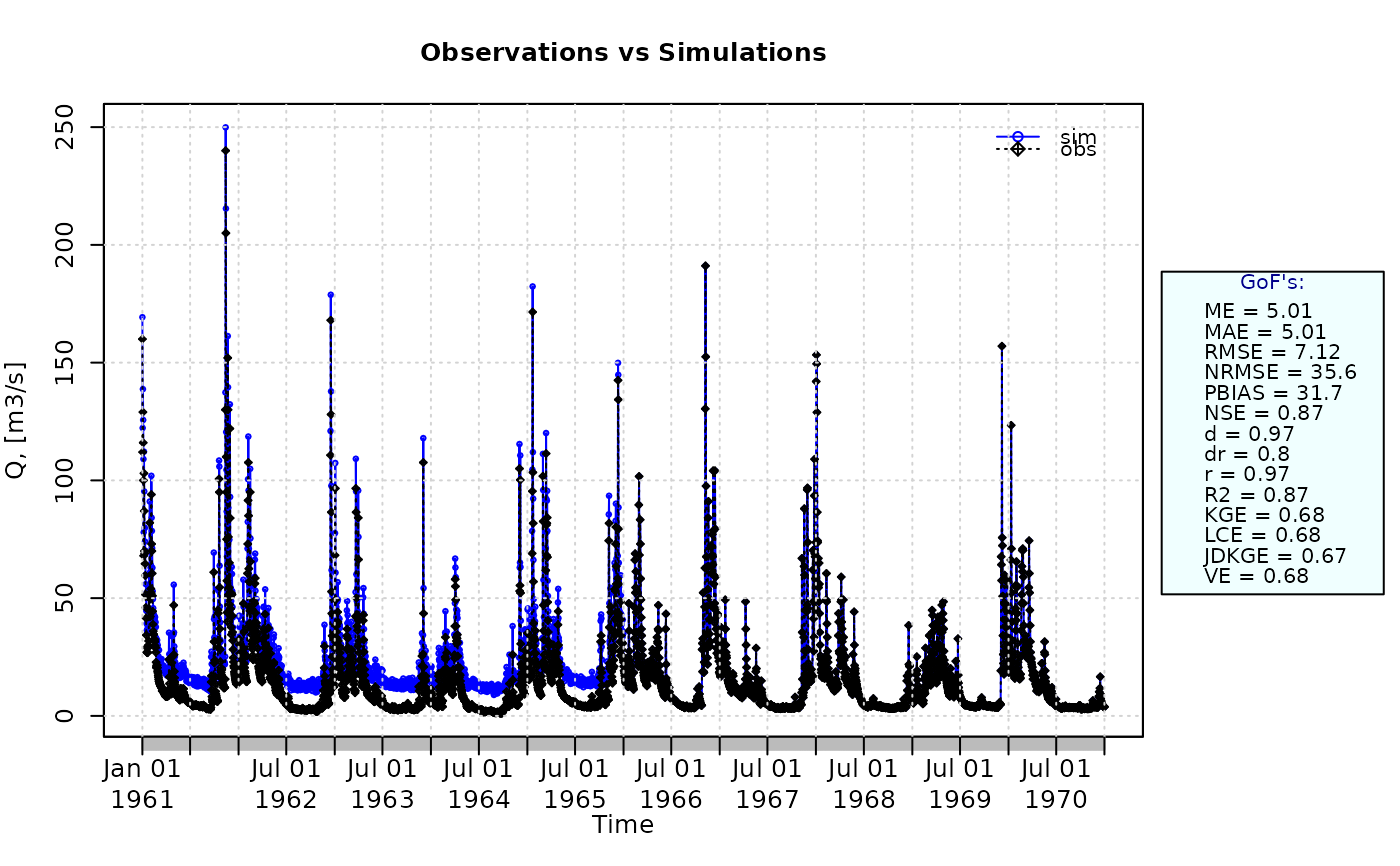LME(sim=sim, obs=obs)
#> [1] 0.6830412

##################
# Example 4: LME for simulated values equal to observations plus random noise 
#            on the first half of the observed values and applying (natural) 
#            logarithm to 'sim' and 'obs' during computations.

LME(sim=sim, obs=obs, fun=log)
#> [1] 0.6666261

# Verifying the previous value:
lsim <- log(sim)
lobs <- log(obs)
LME(sim=lsim, obs=lobs)
#> [1] 0.6666261

##################
# Example 5: LME for simulated values equal to observations plus random noise 
#            on the first half of the observed values and applying (natural) 
#            logarithm to 'sim' and 'obs' and adding the Pushpalatha2012 constant
#            during computations

LME(sim=sim, obs=obs, fun=log, epsilon.type="Pushpalatha2012")
#> [1] 0.6748451

# Verifying the previous value, with the epsilon value following Pushpalatha2012
eps  <- mean(obs, na.rm=TRUE)/100
lsim <- log(sim+eps)
lobs <- log(obs+eps)
LME(sim=lsim, obs=lobs)
#> [1] 0.6748451

##################
# Example 6: LME for simulated values equal to observations plus random noise 
#            on the first half of the observed values and applying (natural) 
#            logarithm to 'sim' and 'obs' and adding a user-defined constant
#            during computations

eps <- 0.01
LME(sim=sim, obs=obs, fun=log, epsilon.type="otherValue", epsilon.value=eps)
#> [1] 0.6671667

# Verifying the previous value:
lsim <- log(sim+eps)
lobs <- log(obs+eps)
LME(sim=lsim, obs=lobs)
#> [1] 0.6671667

##################
# Example 7: LME for simulated values equal to observations plus random noise 
#            on the first half of the observed values and applying (natural) 
#            logarithm to 'sim' and 'obs' and using a user-defined factor
#            to multiply the mean of the observed values to obtain the constant
#            to be added to 'sim' and 'obs' during computations

fact <- 1/50
LME(sim=sim, obs=obs, fun=log, epsilon.type="otherFactor", epsilon.value=fact)
#> [1] 0.6824302

# Verifying the previous value:
eps  <- fact*mean(obs, na.rm=TRUE)
lsim <- log(sim+eps)
lobs <- log(obs+eps)
LME(sim=lsim, obs=lobs)
#> [1] 0.6824302

##################
# Example 8: LME for simulated values equal to observations plus random noise 
#            on the first half of the observed values and applying a 
#            user-defined function to 'sim' and 'obs' during computations

fun1 <- function(x) {sqrt(x+1)}

LME(sim=sim, obs=obs, fun=fun1)
#> [1] 0.7952498

# Verifying the previous value, with the epsilon value following Pushpalatha2012
sim1 <- sqrt(sim+1)
obs1 <- sqrt(obs+1)
LME(sim=sim1, obs=obs1)
#> [1] 0.7952498

##################
# Example 9: LME for a two-column data frame where simulated values are equal to 
#            observations plus random noise on the first half of the observed values 

SIM <- cbind(sim, sim)
OBS <- cbind(obs, obs)

LME(sim=SIM, obs=OBS)
#>       obs       obs 
#> 0.6830412 0.6830412 

##################
# Example 10: LME for each year, where simulated values are given in a two-column data 
#             frame equal to the observations plus random noise on the first half of the 
#             observed values 
SIM <- cbind(sim, sim)
OBS <- cbind(obs, obs)
LME(sim=SIM, obs=OBS, out.PerYear=TRUE)
#>       obs       obs 
#> 0.6830412 0.6830412