Plotting 2 Time Series

Plotting of 2 time series, in two different vertical windows or overlapped in the same window.
It requires the hydroTSM package.

Usage

plot2(x, y, plot.type = "multiple", 
      tick.tstep = "auto", lab.tstep = "auto", lab.fmt=NULL,
      main, xlab = "Time", ylab,
      cal.ini=NA, val.ini=NA, date.fmt="%Y-%m-%d",
      gof.leg = FALSE, gof.digits=2, 
      gofs=c( "ME",  "MAE",  "RMSE", "NRMSE", "PBIAS", "NSE",   "d",    
             "dr",    "r",    "R2",   "KGE",  "LCE", "JDKGE", "VE"),
      legend, leg.cex = 1,
      col = c("black", "blue"),
      cex = c(0.5, 0.5), cex.axis=1.2, cex.lab=1.2, 
      lwd= c(1,1), lty=c(1,3), pch = c(1, 9), 
      pt.style = "ts", add = FALSE, 
      ...)

Arguments

x: time series that will be plotted. class(x) must be ts or zoo. If leg.gof=TRUE, then x is considered as simulated (for some goodness-of-fit functions this is important)
y: time series that will be plotted. class(x) must be ts or zoo. If leg.gof=TRUE, then y is considered as observed values (for some goodness-of-fit functions this is important)
plot.type: character, indicating if the 2 ts have to be plotted in the same window or in two different vertical ones. Valid values are:
-) single : (default) superimposes the 2 ts on a single plot
-) multiple: plots the 2 series on 2 multiple vertical plots
tick.tstep: character, indicating the time step that have to be used for putting the ticks on the time axis. Valid values are: auto, years, months,weeks, days, hours, minutes, seconds.
lab.tstep: character, indicating the time step that have to be used for putting the labels on the time axis. Valid values are: auto, years, months,weeks, days, hours, minutes, seconds.
lab.fmt: Character indicating the format to be used for the label of the axis. See lab.fmt in drawTimeAxis.
main: an overall title for the plot: see title
xlab: label for the 'x' axis
ylab: label for the 'y' axis
cal.ini: OPTIONAL. Character, indicating the date in which the calibration period started.
When cal.ini is provided, all the values in obs and sim with dates previous to cal.ini are SKIPPED from the computation of the goodness-of-fit measures (when gof.leg=TRUE), but their values are still plotted, in order to examine if the warming up period was too short, acceptable or too long for the chosen calibration period. In addition, a vertical red line in drawn at this date.
val.ini: OPTIONAL. Character with the date in which the validation period started.
ONLY used for drawing a vertical red line at this date.
date.fmt: OPTIONAL. Character indicating the format in which the dates entered are stored in cal.ini and val.ini. Default value is %Y-%m-%d. ONLY required when cal.ini or val.ini is provided.
gof.leg: logical, indicating if several numerical goodness-of-fit values have to be computed between sim and obs, and plotted as a legend on the graph. If gof.leg=TRUE (default value), then x is considered as observed and y as simulated values (for some gof functions this is important). This legend is ONLY plotted when plot.type="single"
gof.digits: OPTIONAL, only used when gof.leg=TRUE. Decimal places used for rounding the goodness-of-fit indexes.
gofs: character, with one or more strings indicating the goodness-of-fit measures to be shown in the legend of the plot when gof.leg=TRUE.
Possible values are in c("ME", "MAE", "MSE", "RMSE", "NRMSE", "PBIAS", "RSR", "rSD", "NSE", "mNSE", "rNSE", "d", "md", "rd", "cp", "r", "R2", "bR2", "KGE", "VE").
legend: vector of length 2 to appear in the legend.
leg.cex: numeric, indicating the character expansion factor *relative* to current 'par("cex")'. Used for text, and provides the default for 'pt.cex' and 'title.cex'. Default value = 1
So far, it controls the expansion factor of the 'GoF' legend and the legend referring to x and y
col: character, with the colors of x and y
cex: numeric, with the values controlling the size of text and symbols of x and y with respect to the default
cex.axis: numeric, with the magnification of axis annotation relative to 'cex'. See par.
cex.lab: numeric, with the magnification to be used for x and y labels relative to the current setting of 'cex'. See par.
lwd: vector with the line width of x and y
lty: vector with the line type of x and y
pch: vector with the type of symbol for x and y. (e.g.: 1: white circle; 9: white rhombus with a cross inside)
pt.style: Character, indicating if the 2 ts have to be plotted as lines or bars. Valid values are:
-) ts : (default) each ts is plotted as a lines along the x axis
-) bar: the 2 series are plotted as a barplot.
add: logical indicating if other plots will be added in further calls to this function.
-) FALSE => the plot and the legend are plotted on the same graph
-) TRUE => the legend is plotted in a new graph, usually when called from another function (e.g.: ggof)
...: further arguments passed to plot.zoo function for plotting x, or from other methods

Author

Mauricio Zambrano Bigiarini <mzb.devel@gmail.com>

Note

It requires the package hydroTSM.

Examples

sim <- 2:11
obs <- 1:10
if (FALSE) { # \dontrun{
plot2(sim, obs)
} # }

##################
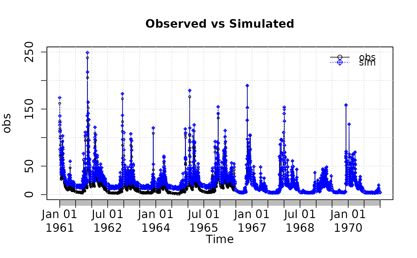
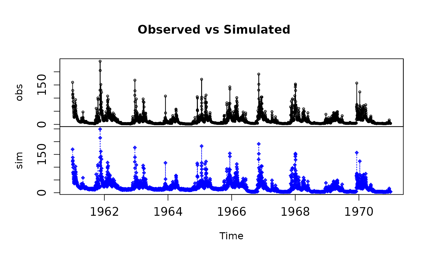
# Loading daily streamflows of the Ega River (Spain), from 1961 to 1970
data(EgaEnEstellaQts)
obs <- EgaEnEstellaQts

# Generating a simulated daily time series, initially equal to the observed series
sim <- obs 

# Randomly changing the first 2000 elements of 'sim', by using a normal distribution 
# with mean 10 and standard deviation equal to 1 (default of 'rnorm').
sim[1:2000] <- obs[1:2000] + rnorm(2000, mean=10)

# Plotting 'sim' and 'obs' in 2 separate panels
plot2(x=obs, y=sim)


# Plotting 'sim' and 'obs' in the same window
plot2(x=obs, y=sim, plot.type="single")

Usage

Arguments

Author

Note

See also

Examples