Theory, computation, and validation of SPI and SPEI with hydroTSM

Mauricio Zambrano-Bigiarini

version 1.1, 27-Jul-2026

Part I: Theoretical background

What SPI and SPEI measure

The Standardized Precipitation Index (SPI) describes how unusual an accumulated precipitation amount is relative to the precipitation climatology for the same location and calendar month. It was introduced as a probability-based, multiscalar index: only precipitation is required, and the accumulation period is selected to represent the memory of the system being studied (McKee et al., 1993; Guttman, 1998; Hayes et al., 1999).

The Standardized Precipitation-Evapotranspiration Index (SPEI) applies the same standardisation principle to climatic water balance,

$$D_t = P_t - PET_t,$$

where $P_t$ is precipitation and $PET_t$ is potential evapotranspiration. Consequently, SPEI responds both to water supply and to atmospheric evaporative demand. This makes it useful when temperature variability or long-term warming affects drought severity, but also makes the result sensitive to the selected PET method and the quality of its meteorological inputs (Vicente-Serrano et al., 2010; Beguería et al., 2014).

For either index, let $X_t$ denote monthly precipitation for SPI or monthly water balance for SPEI. A backward-looking value at scale $k$ is

$$Y_{t,k} = \sum_{j=0}^{k-1} w_j X_{t-j},$$

where $w_j$ are the kernel weights. A separate probability distribution $F_m$ is fitted to $Y_{t,k}$ for each calendar month $m$, because a January water balance should be compared with other Januaries rather than with months from a different season. The fitted non-exceedance probability is then mapped to a standard-normal variate:

$$I_{t,k} = \Phi^{-1}\{H_m(Y_{t,k})\},$$

where $\Phi^{-1}$ is the standard-normal quantile function and $H_m$ is either the fitted continuous distribution or, for zero precipitation, a mixed discrete-continuous distribution. If the probability model is well calibrated, the resulting index has an approximately standard-normal interpretation: zero is near the climatological median, negative values are drier than normal, and positive values are wetter than normal. Standard-normal thresholds of -1, -1.5, and -2 correspond approximately to lower-tail probabilities of 15.9%, 6.7%, and 2.3%, respectively.

SPI and SPEI describe statistical rarity, not drought impact by themselves. The same index value can have different consequences depending on season, exposure, water storage, crop stage, and antecedent conditions.

Temporal scales and system memory

The scale is the number of current and preceding months contributing to each index value. It is not the duration of an identified drought event. A drought event may persist for many index values, and neighbouring values are correlated because their accumulation windows overlap.

Common interpretations are:

• 1 month: immediate precipitation or water-balance anomaly and rapidly developing meteorological drought;
• 3 months: short seasonal conditions, soil-moisture stress, and rain-fed agricultural response;
• 6 months: seasonal water availability and slower agricultural or surface-water response;
• 12 months: annual water balance, streamflow, reservoir, and groundwater signals; and
• 24 months or longer: persistent hydrological storage deficits.

These are guidelines, not universal definitions. The appropriate scale should be selected against the response time of the variable or impact of interest. Multiscalar interpretation is one of the principal advantages of both indices (Guttman, 1998; Vicente-Serrano et al., 2010). Comparing several scales is often more informative than choosing a single scale in advance.

Why distribution choice matters

The probability model determines the percentile assigned to each accumulated value and therefore directly controls the final index, especially in the tails. A poor distribution can exaggerate or suppress drought severity even when the fitted mean appears reasonable (Stagge et al., 2015). Distribution choice should respect both the support of the data and the empirical shape:

• SPI precipitation is non-negative, usually right-skewed at short scales, and may contain an exact probability mass at zero. Skewness commonly decreases with longer accumulation.
• SPEI water balance can be negative or positive, so distributions with a location parameter and support extending below zero are generally required.

Stagge et al. (2015) evaluated seven SPI candidates (Gamma, Gumbel, logistic, log-logistic, lognormal, normal, and Weibull) and four SPEI candidates (generalized logistic, GEV, normal, and Pearson type III). They found the two-parameter Gamma to be a strong general SPI choice in their European experiment and recommended GEV for SPEI there. The original SPEI formulation used the three-parameter log-logistic distribution, which is represented here by the equivalent generalized-logistic formulation (Vicente-Serrano et al., 2010). These findings should not be treated as universal winners: performance can change with climate, record length, calendar month, accumulation scale, and observational or modelled data (Pieper et al., 2020).

A defensible selection checks every calendar month and scale, with particular attention to the dry tail. Useful diagnostics include Q-Q or P-P plots, empirical versus theoretical drought-category frequencies, tail-sensitive goodness-of-fit statistics, and validation outside the calibration period. Goodness-of-fit critical values must account for estimated parameters; applying an ordinary Kolmogorov-Smirnov reference distribution after fitting parameters to the same sample is not valid without adjustment or resampling.

Why parameter-estimation method matters

Distribution family and parameter estimator are separate decisions. Two implementations can use the same named distribution but produce different indices because their parameter estimates differ.

• Maximum likelihood (fit="max-lik") selects parameters that maximise the probability of the calibration sample. Under a correct model and standard regularity conditions it is statistically efficient, but it can be sensitive to starting values, outliers, parameter boundaries, and small samples.
• Unbiased probability-weighted moments (fit="ub-pwm") estimate moments that combine observations with their non-exceedance probabilities using unbiased order-statistic weights. PWMs and the related L-moments provide stable estimators for many skewed hydrological distributions (Greenwood et al., 1979; Hosking, 1990). Beguería et al. (2014) recommend unbiased PWM for the SPEI log-logistic model.
• Plotting-position PWM (fit="pp-pwm") replaces the unknown probabilities by empirical plotting positions. hydroTSM uses $F_i=(i-0.35)/n$, matching the constants used by the SPEI package. This was used in the original SPEI formulation, but it is not identical to unbiased PWM and can differ appreciably in the short monthly calibration samples.

There is no estimator that compensates for a badly chosen distribution. Selection should consider convergence, plausibility of parameters, fit in the tails, and sensitivity of the resulting drought classes. Comparisons between packages are fair only when distribution, estimator, accumulation, reference period, zero treatment, and scaling conventions are equivalent.

Theoretical guide to the function arguments

The arguments below separate scientific choices from numerical and output controls. Defaults are intentionally stated because hydroTSM defaults do not always match those of other R packages.

Data, accumulation, and calibration

argument	applies.to	values.and.default
x	SPI and SPEI	Numeric monthly zoo series; precipitation for SPI and P - PET for SPEI. The index must be Date, POSIXt, or yearmon and months must be consecutive.
scale	SPI and SPEI	Any positive integer not exceeding the series length; no default. It controls the backward-looking memory and must be provided explicitly.
kernel	SPI and SPEI	list(type, shift); type is rectangular, triangular, circular, or gaussian and shift is 0,…,scale-1. Default list(type=‘rectangular’, shift=0).
ref.start, ref.end	SPI and SPEI	NULL, a Date object, or a character string in YYYY-MM or YYYY-MM-DD format; both default to NULL, which fits the full record. They define the climatology used for parameter estimation, not the output period.
zero.threshold	SPI only	Any finite non-negative number; default 0. Values strictly below it become zero before accumulation, allowing a trace-precipitation definition.
p0	SPI and SPEI	TRUE or FALSE; defaults TRUE for SPI and FALSE for SPEI. TRUE represents exact zeros by a point mass plus a continuous positive distribution.
p0.center.mass	SPI and SPEI	TRUE or FALSE; default FALSE. With p0=TRUE, TRUE assigns zeros to the centre of their empirical probability mass rather than its upper edge.

The kernel encodes how memory is distributed within the selected scale. "rectangular" gives all months equal weight. The other kernels progressively change the relative influence of older observations, while shift moves the weighting pattern within the backward-looking window. A non-rectangular kernel therefore changes the scientific meaning of the index and should be justified by the response dynamics being represented.

The reference period defines “normal”. A short period produces uncertain tail parameters because each calendar-month fit has approximately one observation per reference year. A changing reference period also changes the climatology against which drought is measured, so fixed and moving references answer different questions.

Distribution and parameter estimation

argument	applies.to	values.and.default
distribution	SPI and SPEI	SPI: gamma (default), gumbel, logis, llogis, lnorm, norm, or weibull. SPEI: genlog (default), gev, norm, or pe3.
fit	SPI and SPEI	max-lik (default), ub-pwm, or pp-pwm. It selects how each calendar month’s distribution parameters are estimated.
params	SPI and SPEI	NULL (default), a parameter vector, an npar x 12 matrix, or an npar x nseries x 12 array. Supplied values define a fixed probability model and bypass fitting.
start.fun	SPI and SPEI	NULL (default) or function(x, distr). It supplies starting parameters to maximum-likelihood optimisation for each month and series.
start.fun.fix	SPI and SPEI	TRUE or FALSE; default FALSE. TRUE substitutes starting estimates when optimisation fails; this improves continuity but does not constitute a converged MLE.
scaling	SPI and SPEI	sd (default), no, or max. Accumulated data are divided by their standard deviation, left unchanged, or divided by their maximum before fitting to improve numerical conditioning.
…	SPI and SPEI	Optional maximum-likelihood controls, principally mledist.par, such as optimiser, bounds, fixed parameters, and optimiser-specific controls.

params is appropriate when parameters have been estimated externally, when a common climatology must be applied consistently, or when an operational system must not refit retrospectively. Supplied parameters must use the parameter order and convention documented in ?spi; they apply to unscaled accumulated data. Therefore, fit, scaling, start.fun, and start.fun.fix no longer affect the result when params is supplied.

The accepted parameter names and order are: gamma=(shape, rate), gumbel=(loc, scale), logis=(location, scale), llogis=(shape, scale), lnorm=(meanlog, sdlog), norm=(mean, sd), weibull=(shape, scale), genlog=(shape, scale, location), gev=(loc, scale, shape), and pe3=(shape, scale, location). Scale and standard-deviation parameters must be positive; additional distribution-specific constraints are checked by the function.

scaling is a numerical conditioning device, not a change to drought theory. With internally estimated location/scale families, consistent rescaling should not materially alter the standardised probabilities. It does matter to optimisation stability and must not be mixed with parameter values calibrated on a different scale.

Missing values, bounds, and returned objects

argument	applies.to	values.and.default
sci.limit	SPI and SPEI	Any non-negative number, including Inf (default). Finite values truncate the final index symmetrically to [-sci.limit, sci.limit].
na.rm	SPI and SPEI	TRUE or FALSE; default FALSE. TRUE omits missing calibration values during fitting, but an accumulation window containing NA remains NA.
out.type	SPI and SPEI	zoo (default) or numeric. zoo preserves the time index and column names; numeric returns a vector or matrix.
verbose	SPI and SPEI	TRUE or FALSE; default FALSE. TRUE emits bracketed progress messages and does not change the calculation.
warn	SPI and SPEI	TRUE or FALSE; default TRUE. FALSE suppresses fitting and transformation warnings but does not repair failed estimates.

Finite sci.limit values can prevent unstable extrapolation from producing implausibly large magnitudes in a short calibration record (Stagge et al., 2015). Truncation is a reporting safeguard, not an uncertainty estimate: several observations can be assigned the same bound, and the true tail probability remains uncertain.

Part II: Practical use and package comparisons

The spi() and spei() functions calculate standardized drought indices from complete monthly zoo series. Their production calculations use base R and do not require the SCI, SPEI, or lmomco packages.

This practical part has two goals:

1. explain the main hydroTSM workflows for SPI and SPEI; and
2. document reproducible comparisons with SCI and SPEI at accumulation scales 1, 3, 6, and 12.

The comparison section distinguishes equivalent computations from comparisons that use different fitting methods or zero-frequency treatments. A high correlation in a non-equivalent comparison is useful descriptive information, but is not evidence of numerical reproduction under identical conditions.

Differences from the SPEI and SCI packages

At the time of this benchmark, the CRAN versions were SPEI 1.8.1 and SCI 1.0-3. The comparison below concerns their documented public interfaces and the hydroTSM 0.8-8 implementation, rather than suggesting that one design is preferable for every workflow.

aspect	hydroTSM	SPEI 1.8.1	SCI 1.0-3
Primary interface	Direct spi() and spei() functions.	Direct spi() and spei(); spi() is a wrapper around spei().	Separate fitSCI() and transformSCI() steps.
Input and result	Consecutive monthly zoo input; returns zoo or numeric values directly.	Vector, matrix, data frame, or ts-like input; returns a spei object with fitted values and coefficients.	Default methods operate on a monthly numeric univariate series plus first.mon; transformation returns numeric values.
Default calculation	scale is required; Gamma/p0 for SPI, genlog/no p0 for SPEI; max-lik fitting.	scale is required; Gamma for SPI, log-Logistic for SPEI; ub-pwm fitting.	time.scale, distribution, and p0 are explicit; fitting is maximum likelihood.
Distributions	All seven SPI and four SPEI candidates evaluated by Stagge et al. (2015).	Gamma, log-Logistic, and PearsonIII in the drought-index interface.	General SCI engine; bundled starting estimators cover nine named distributions and custom distributions can be supplied.
Parameter estimation	max-lik, ub-pwm, and pp-pwm; custom starts, fallback starts, or supplied parameters.	ub-pwm, pp-pwm, and max-lik labels; available behaviour depends on distribution and data; supplied parameters supported.	Maximum likelihood with L-moment/moment starting estimates and custom start/fallback controls.
Zero and tail controls	zero.threshold for SPI; p0, centred zero mass, and symmetric sci.limit for either wrapper.	The spi()/spei() signatures do not expose zero.threshold, centred-zero-mass, or sci.limit controls.	p0, centred zero mass, scaling, and sci.limit are explicit; no zero.threshold argument.
PET calculation	Expects P - PET for spei(); PET must be computed separately.	Package includes Thornthwaite, Hargreaves, and Penman PET functions.	Expects the climate variable or P - PET to be prepared separately.
Fitted-model information	Returns the index, not a fitted-model object.	Returns coefficients, fitted values, settings, and optional input in a spei object.	fitSCI() returns monthly parameters and diagnostic flags for later transformation.
Runtime dependencies	Distribution fitting and optimisation use base R; no SCI, SPEI, lmomco, fitdistrplus, or evd dependency.	Imports lmomco, lmom, TLMoments, reshape, ggplot2, checkmate, zoo, and lubridate.	Depends on fitdistrplus and lmomco; evd is suggested.

The most important comparison consequence is the estimator default: hydroTSM uses maximum likelihood, whereas SPEI defaults to unbiased PWM and SCI fits by maximum likelihood. Equivalent numerical comparisons must therefore set fit explicitly. The generalized-logistic model used by hydroTSM and SCI for SPEI is functionally equivalent to the three-parameter log-logistic formulation used by the SPEI package, but parameter names and signs must be mapped consistently when parameters are supplied.

The current CRAN package descriptions and manuals are available at https://CRAN.R-project.org/package=SPEI and https://CRAN.R-project.org/package=SCI.

Basic usage

library(hydroTSM)
#> Loading required package: zoo
#> 
#> Attaching package: 'zoo'
#> The following objects are masked from 'package:base':
#> 
#>     as.Date, as.Date.numeric

The main argument is a numeric monthly zoo object with a Date, POSIXt, or yearmon index. The observations must cover consecutive months.

The following example uses monthly precipitation from one station in the EbroPPtsMonthly dataset.

data(EbroPPtsMonthly)

pcp <- zoo::zoo(EbroPPtsMonthly$P9001, EbroPPtsMonthly$Date)
head(pcp)
#> 1941-01-01 1941-02-01 1941-03-01 1941-04-01 1941-05-01 1941-06-01 
#>      311.6      158.9       91.2       39.5      135.3       41.7

SPI

scale must be provided explicitly. With scale=12, spi() uses a Gamma distribution, maximum-likelihood parameter estimation, and a mixed probability at zero:

spi12 <- spi(pcp, scale=12, warn=FALSE)
head(spi12, 15)
#> 1941-01-01 1941-02-01 1941-03-01 1941-04-01 1941-05-01 1941-06-01 1941-07-01 1941-08-01 
#>         NA         NA         NA         NA         NA         NA         NA         NA 
#> 1941-09-01 1941-10-01 1941-11-01 1941-12-01 1942-01-01 1942-02-01 1942-03-01 
#>         NA         NA         NA  1.4114490  0.7628638  0.7692549  1.0063587

The accumulation scale is changed with scale. Trace precipitation can be treated as zero before accumulation with zero.threshold:

spi1 <- spi(pcp, scale=1, zero.threshold=0.1, warn=FALSE)
spi3 <- spi(pcp, scale=3, zero.threshold=0.1, warn=FALSE)
spi6 <- spi(pcp, scale=6, zero.threshold=0.1, warn=FALSE)

The controls for low and zero precipitation have separate purposes:

• zero.threshold changes monthly values strictly below the threshold to zero;
• p0=TRUE uses a mixed distribution with a point probability at zero;
• p0.center.mass=TRUE uses the centered zero-mass estimator; and
• sci.limit bounds the final standardized index.

For example:

spi3.bounded <- spi(
  pcp, scale=3, zero.threshold=0.1,
  p0=TRUE, p0.center.mass=TRUE,
  sci.limit=3, warn=FALSE
)
range(spi3.bounded, na.rm=TRUE)
#> [1] -2.367121  2.035581

SPEI

spei() expects monthly climatic water balance, normally precipitation minus potential evapotranspiration. Its defaults select the generalized-logistic distribution and do not use a zero-probability mixture.

For illustration, a deterministic seasonal PET series is constructed below:

month.number <- as.integer(format(zoo::index(pcp), "%m"))
pet <- zoo::zoo(
  60 + 35 * sin(2 * pi * (month.number - 1) / 12),
  zoo::index(pcp)
)
water.balance <- pcp - pet

spei3 <- spei(water.balance, scale=3, warn=FALSE)
head(spei3)
#> 1941-01-01 1941-02-01 1941-03-01 1941-04-01 1941-05-01 1941-06-01 
#>         NA         NA  1.6907612  0.3953445  0.6236039  0.4519379

SPI and SPEI retain the input time index. Initial values are NA when a complete accumulation window is not yet available.

indices <- zoo::merge.zoo(SPI=spi3, SPEI=spei3)
plot(
  indices, plot.type="single", col=c("#1b9e77", "#d95f02"), lwd=1.2,
  xlab="Date", ylab="Standardized drought index"
)
abline(h=c(-2, -1, 0, 1, 2), col="grey85", lty=c(3, 3, 1, 3, 3))
legend(
  "topright", legend=colnames(indices),
  col=c("#1b9e77", "#d95f02"), lty=1, lwd=1.2, bty="n"
)

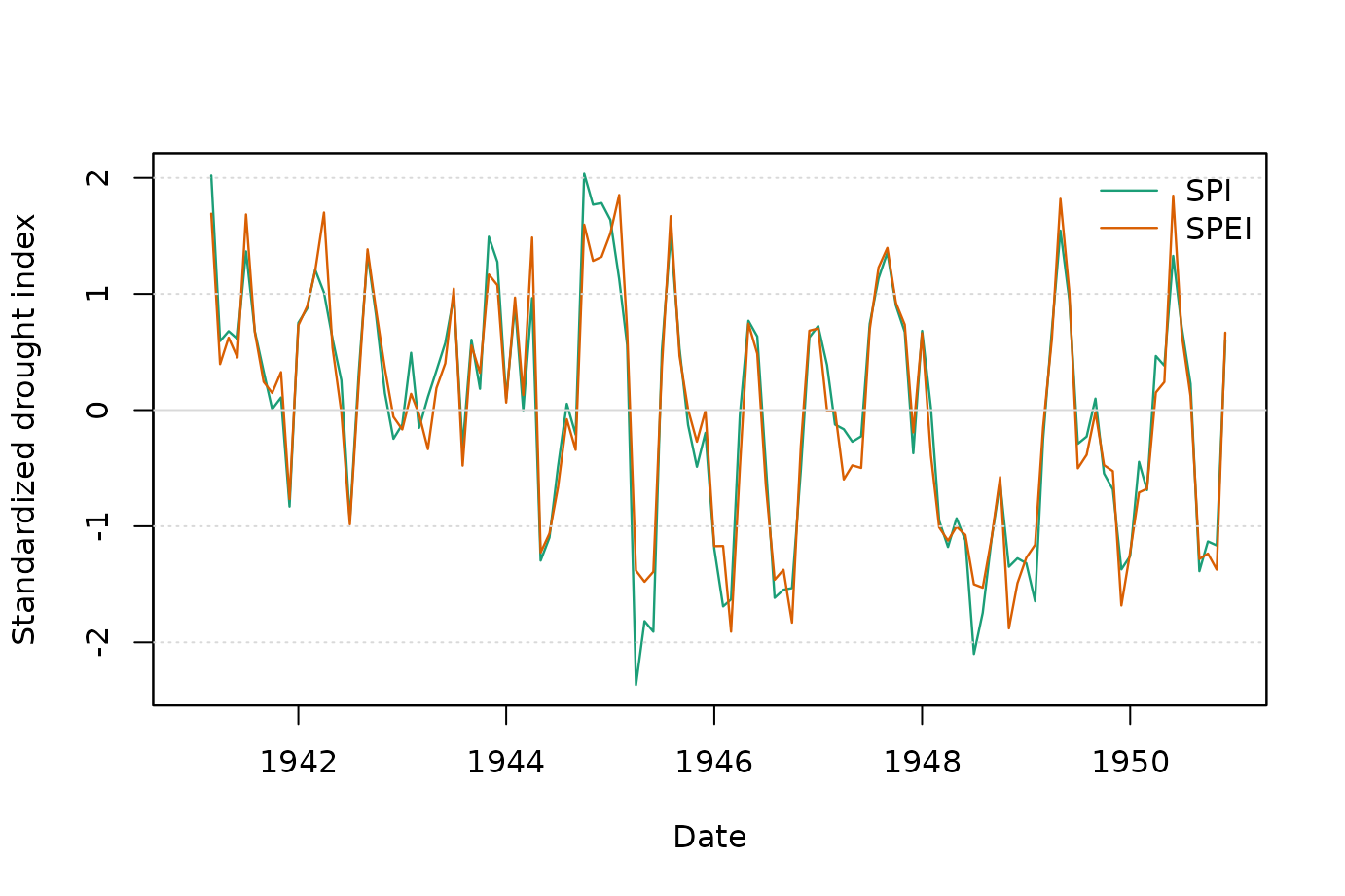
Figure 1. Example three-month SPI and SPEI series.

Distributions and parameter estimation

The supported distributions are those evaluated for SPI and SPEI by Stagge et al. (2015). The parameter column shows the required order when params is supplied without names.

argument	distribution	parameters
gamma	Gamma	shape, rate
gumbel	Gumbel	loc, scale
logis	logistic	location, scale
llogis	log-logistic	shape, scale
lnorm	lognormal	meanlog, sdlog
norm	normal	mean, sd
weibull	Weibull	shape, scale

argument	distribution	parameters
genlog	generalized logistic	shape, scale, location
gev	GEV	loc, scale, shape
norm	normal	mean, sd
pe3	Pearson type III	shape, scale, location

Three estimation methods are available:

• fit="max-lik": maximum likelihood;
• fit="ub-pwm": unbiased probability-weighted moments; and
• fit="pp-pwm": plotting-position probability-weighted moments.

For example:

spi3.mle <- spi(pcp, scale=3, fit="max-lik", warn=FALSE)
spi3.ub  <- spi(pcp, scale=3, fit="ub-pwm", warn=FALSE)
spi3.pp  <- spi(pcp, scale=3, fit="pp-pwm", warn=FALSE)

Reference periods

Distribution parameters can be calibrated over a subperiod and then applied to the complete series:

spi3.reference <- spi(
  pcp, scale=3,
  ref.start="1943-01", ref.end="1948-12",
  warn=FALSE
)

Accumulation is performed before the reference-period subset is selected. Therefore, an accumulated value at the start of the reference period can use earlier observations from x. Character references can also include a day, for example "1943-01-01", or be supplied as Date objects. The day component is only used to identify the calendar month.

Supplied parameters

params bypasses parameter fitting. It accepts:

• a vector reused for every calendar month and series;
• an npar by 12 matrix of monthly parameters, reused for every series; or
• an npar by nseries by 12 array.

Named parameters are reordered automatically. Supplied parameters refer to the unscaled accumulated data, so scaling is ignored.

Vector example: the same normal parameter set is reused for every calendar month and every series.

spei.fixed.vector <- spei(
  water.balance, scale=1, distribution="norm",
  params=c(mean=0, sd=40), warn=FALSE
)
head(spei.fixed.vector)
#>  1941-01-01  1941-02-01  1941-03-01  1941-04-01  1941-05-01  1941-06-01 
#>  6.28999996  2.03500000  0.02222777 -1.38750000  1.12472777 -0.89500000

Matrix example: each calendar month receives its own parameter set, reused for all series.

monthly.normal.params <- rbind(
  mean=seq(-10, 10, length.out=12),
  sd=rep(40, 12)
)
spei.fixed.monthly <- spei(
  water.balance, scale=1, distribution="norm",
  params=monthly.normal.params, warn=FALSE
)
head(spei.fixed.monthly)
#> 1941-01-01 1941-02-01 1941-03-01 1941-04-01 1941-05-01 1941-06-01 
#>  6.5400001  2.2395455  0.1813187 -1.2738636  1.1929096 -0.8722727

Array example: each series and calendar month receives its own parameter set.

water.balance.two <- zoo::merge.zoo(
  stationA=water.balance,
  stationB=water.balance + 5
)
array.normal.params <- array(
  NA_real_, dim=c(2, 2, 12),
  dimnames=list(c("mean", "sd"), colnames(water.balance.two), month.abb)
)
array.normal.params["mean", "stationA", ] <- 0
array.normal.params["mean", "stationB", ] <- 5
array.normal.params["sd", , ] <- 40

spei.fixed.array <- spei(
  water.balance.two, scale=1, distribution="norm",
  params=array.normal.params, warn=FALSE
)
head(spei.fixed.array)
#>               stationA    stationB
#> 1941-01-01  6.28999996  6.28999996
#> 1941-02-01  2.03500000  2.03500000
#> 1941-03-01  0.02222777  0.02222777
#> 1941-04-01 -1.38750000 -1.38750000
#> 1941-05-01  1.12472777  1.12472777
#> 1941-06-01 -0.89500000 -0.89500000

For SPI, p0=TRUE still estimates the monthly zero probability from the reference data when continuous-distribution parameters are supplied.

Custom maximum-likelihood starting values

start.fun follows the SCI interface and is called once for each calendar month and series as start.fun(x, distr). The default NULL uses hydroTSM’s internal base-R estimator.

normal.start <- function(x, distr) {
  c(mean=mean(x), sd=stats::sd(x))
}

spei3.custom <- spei(
  water.balance, scale=3, distribution="norm",
  fit="max-lik", start.fun=normal.start,
  start.fun.fix=FALSE, warn=FALSE
)

When optimization fails, start.fun.fix=FALSE returns NA for the affected month. Setting it to TRUE retains the initial values, which may be useful for continuity but should not be interpreted as a converged maximum-likelihood fit.

Progress messages

verbose=TRUE emits bracketed messages:

invisible(spi(pcp, scale=3, fit="ub-pwm", verbose=TRUE, warn=FALSE))
#> [SPI: scale=3; distribution=gamma; fit=ub-pwm; kernel=rectangular; shift=0]
#> [SPI: reference period 1941-01 to 1950-12]
#> [SPI: processing series 1 of 1 (1)]
#> [SPI: computation completed]

Comparison design

The objective is to compare the SPI and SPEI series computed by the current hydroTSM implementation with series computed by the SPEI and SCI packages. The comparisons are made independently for accumulation scales 1, 3, 6, and 12 and for hydroTSM fit="max-lik", fit="pp-pwm", and fit="ub-pwm".

The benchmark uses the Wichita monthly dataset distributed with SPEI. Climatic water balance was calculated with Thornthwaite PET at latitude 37.6475 degrees north. All implementations used a rectangular kernel and the full record.

The package versions and data period used to create the bundled benchmark are:

field	value
generated	2026-07-27
hydroTSM	0.8-8
SCI	1.0.3
SPEI	1.8.1
R	4.6.0
data	SPEI::wichita
period	1980-01 to 2011-10
observations	382
PET	Thornthwaite; latitude 37.6475 degrees north

All tables and plots use hydroTSM as the first series. The benchmark uses:

• Gamma with mixed zero probability for SPI;
• generalized logistic/log-logistic for SPEI;
• scaling="sd" for hydroTSM and SCI;
• scales 1, 3, 6, and 12; and
• all three hydroTSM fitting methods.

SCI supplies the maximum-likelihood reference. It has no fit argument corresponding to hydroTSM’s PWM alternatives, so comparisons of SCI with ub-pwm or pp-pwm are descriptive rather than equivalent.

For SPEI 1.8.1, the same fit argument was requested from the package. ub-pwm produced finite results. In this dataset, the max-lik and pp-pwm runs produced no finite index values, so those cases are reported as not computable rather than assigned an artificial error statistic.

At scale 1, Wichita contains exact zero precipitation. The two packages treat those zero values differently in this configuration, so the scale-1 SPI comparison with SPEI is not fully equivalent. At scales 3, 6, and 12 there are no zero accumulated totals and the ub-pwm Gamma comparison is equivalent.

Accuracy measures

Metrics are calculated only where both series are finite:

• correlation measures linear agreement;
• RMSE is the root mean squared difference;
• MAE is the mean absolute difference; and
• maximum error is the largest absolute difference.

Independent comparison tables

Each table fixes one hydroTSM index and one hydroTSM fitting method, then compares that hydroTSM series separately with SCI and SPEI at scales 1, 3, 6, and 12. The hydroTSM result column identifies the series produced by the current hydroTSM function. The reference result column identifies the external package series used as the comparator. Both columns state the package, index, distribution, and fitting method.

The status column identifies the conditions behind each row. Fair means the distribution, fitting method, accumulation, reference period, scaling convention, and zero treatment are equivalent for the comparison being made. Other status values identify why the row is descriptive rather than a strict reproduction test. The nonfinite hydroTSM/reference column reports the number of non-finite values in each input series before pairwise metrics are calculated.

SPI: fit="max-lik"

Rows use the full Wichita record, a rectangular kernel, scaling="sd" for hydroTSM and SCI, and the distribution named in the result columns.

scale	hydroTSM result	reference result	status	pairs	correlation	RMSE	MAE	max.error	nonfinite hydroTSM/reference
1	hydroTSM; SPI; gamma; max-lik	SCI; SPI; gamma; max-lik	Fair	382	1.0000000	0.0001519	0.0001113	0.0006126	0 / 0
1	hydroTSM; SPI; gamma; max-lik	SPEI; SPI; Gamma; max-lik	No finite reference values	0	NA	NA	NA	NA	0 / 382
3	hydroTSM; SPI; gamma; max-lik	SCI; SPI; gamma; max-lik	Fair	380	0.9999999	0.0003499	0.0002739	0.0010764	2 / 2
3	hydroTSM; SPI; gamma; max-lik	SPEI; SPI; Gamma; max-lik	No finite reference values	0	NA	NA	NA	NA	2 / 382
6	hydroTSM; SPI; gamma; max-lik	SCI; SPI; gamma; max-lik	Fair	377	0.9999993	0.0012310	0.0007004	0.0063191	5 / 5
6	hydroTSM; SPI; gamma; max-lik	SPEI; SPI; Gamma; max-lik	No finite reference values	0	NA	NA	NA	NA	5 / 382
12	hydroTSM; SPI; gamma; max-lik	SCI; SPI; gamma; max-lik	Fair	371	0.9999996	0.0009383	0.0006992	0.0036331	11 / 11
12	hydroTSM; SPI; gamma; max-lik	SPEI; SPI; Gamma; max-lik	No finite reference values	0	NA	NA	NA	NA	11 / 382
1	hydroTSM; SPI; gamma; pp-pwm	SCI; SPI; gamma; max-lik	Different fitting methods	382	0.9945497	0.1107620	0.0716189	0.4216345	0 / 0
1	hydroTSM; SPI; gamma; pp-pwm	SPEI; SPI; Gamma; pp-pwm	No finite reference values	0	NA	NA	NA	NA	0 / 382
3	hydroTSM; SPI; gamma; pp-pwm	SCI; SPI; gamma; max-lik	Different fitting methods	380	0.9994337	0.0350645	0.0232709	0.1514544	2 / 2
3	hydroTSM; SPI; gamma; pp-pwm	SPEI; SPI; Gamma; pp-pwm	No finite reference values	0	NA	NA	NA	NA	2 / 382
6	hydroTSM; SPI; gamma; pp-pwm	SCI; SPI; gamma; max-lik	Different fitting methods	377	0.9990121	0.0446591	0.0299962	0.1928399	5 / 5
6	hydroTSM; SPI; gamma; pp-pwm	SPEI; SPI; Gamma; pp-pwm	No finite reference values	0	NA	NA	NA	NA	5 / 382
12	hydroTSM; SPI; gamma; pp-pwm	SCI; SPI; gamma; max-lik	Different fitting methods	371	0.9991394	0.0473254	0.0318784	0.1705649	11 / 11
12	hydroTSM; SPI; gamma; pp-pwm	SPEI; SPI; Gamma; pp-pwm	No finite reference values	0	NA	NA	NA	NA	11 / 382
1	hydroTSM; SPI; gamma; ub-pwm	SCI; SPI; gamma; max-lik	Different fitting methods	382	0.9944339	0.1086218	0.0722700	0.4317486	0 / 0
1	hydroTSM; SPI; gamma; ub-pwm	SPEI; SPI; Gamma; ub-pwm	Different zero treatment	378	0.9978624	0.0710284	0.0220714	0.7196583	0 / 4
3	hydroTSM; SPI; gamma; ub-pwm	SCI; SPI; gamma; max-lik	Different fitting methods	380	0.9994135	0.0344074	0.0225190	0.1973298	2 / 2
3	hydroTSM; SPI; gamma; ub-pwm	SPEI; SPI; Gamma; ub-pwm	Fair	380	1.0000000	0.0000000	0.0000000	0.0000000	2 / 2
6	hydroTSM; SPI; gamma; ub-pwm	SCI; SPI; gamma; max-lik	Different fitting methods	377	0.9990477	0.0464925	0.0262307	0.2710078	5 / 5
6	hydroTSM; SPI; gamma; ub-pwm	SPEI; SPI; Gamma; ub-pwm	Fair	377	1.0000000	0.0000000	0.0000000	0.0000000	5 / 5
12	hydroTSM; SPI; gamma; ub-pwm	SCI; SPI; gamma; max-lik	Different fitting methods	371	0.9991450	0.0443540	0.0271500	0.2698663	11 / 11
12	hydroTSM; SPI; gamma; ub-pwm	SPEI; SPI; Gamma; ub-pwm	Fair	371	1.0000000	0.0000000	0.0000000	0.0000000	11 / 11
1	hydroTSM; SPEI; genlog; max-lik	SCI; SPEI; genlog; max-lik	Fair	382	1.0000000	0.0000000	0.0000000	0.0000000	0 / 0
1	hydroTSM; SPEI; genlog; max-lik	SPEI; SPEI; log-Logistic; max-lik	No finite reference values	0	NA	NA	NA	NA	0 / 382
3	hydroTSM; SPEI; genlog; max-lik	SCI; SPEI; genlog; max-lik	Fair	380	1.0000000	0.0001508	0.0001193	0.0004576	2 / 2
3	hydroTSM; SPEI; genlog; max-lik	SPEI; SPEI; log-Logistic; max-lik	No finite reference values	0	NA	NA	NA	NA	2 / 382
6	hydroTSM; SPEI; genlog; max-lik	SCI; SPEI; genlog; max-lik	Fair	377	1.0000000	0.0001518	0.0001153	0.0009990	5 / 5
6	hydroTSM; SPEI; genlog; max-lik	SPEI; SPEI; log-Logistic; max-lik	No finite reference values	0	NA	NA	NA	NA	5 / 382
12	hydroTSM; SPEI; genlog; max-lik	SCI; SPEI; genlog; max-lik	Fair	371	1.0000000	0.0001156	0.0000931	0.0003654	11 / 11
12	hydroTSM; SPEI; genlog; max-lik	SPEI; SPEI; log-Logistic; max-lik	No finite reference values	0	NA	NA	NA	NA	11 / 382
1	hydroTSM; SPEI; genlog; pp-pwm	SCI; SPEI; genlog; max-lik	Different fitting methods	382	0.9944417	0.1114665	0.0733363	0.6208688	0 / 0
1	hydroTSM; SPEI; genlog; pp-pwm	SPEI; SPEI; log-Logistic; pp-pwm	No finite reference values	0	NA	NA	NA	NA	0 / 382
3	hydroTSM; SPEI; genlog; pp-pwm	SCI; SPEI; genlog; max-lik	Different fitting methods	380	0.9986465	0.0625231	0.0446514	0.3408091	2 / 2
3	hydroTSM; SPEI; genlog; pp-pwm	SPEI; SPEI; log-Logistic; pp-pwm	No finite reference values	0	NA	NA	NA	NA	2 / 382
6	hydroTSM; SPEI; genlog; pp-pwm	SCI; SPEI; genlog; max-lik	Different fitting methods	377	0.9989651	0.0558998	0.0448326	0.1819346	5 / 5
6	hydroTSM; SPEI; genlog; pp-pwm	SPEI; SPEI; log-Logistic; pp-pwm	No finite reference values	0	NA	NA	NA	NA	5 / 382
12	hydroTSM; SPEI; genlog; pp-pwm	SCI; SPEI; genlog; max-lik	Different fitting methods	371	0.9993944	0.0395628	0.0303868	0.1788221	11 / 11
12	hydroTSM; SPEI; genlog; pp-pwm	SPEI; SPEI; log-Logistic; pp-pwm	No finite reference values	0	NA	NA	NA	NA	11 / 382
1	hydroTSM; SPEI; genlog; ub-pwm	SCI; SPEI; genlog; max-lik	Different fitting methods	382	0.9932742	0.1182039	0.0686749	0.6962337	0 / 0
1	hydroTSM; SPEI; genlog; ub-pwm	SPEI; SPEI; log-Logistic; ub-pwm	Fair	382	1.0000000	0.0000000	0.0000000	0.0000000	0 / 0
3	hydroTSM; SPEI; genlog; ub-pwm	SCI; SPEI; genlog; max-lik	Different fitting methods	380	0.9980837	0.0631107	0.0399493	0.3337133	2 / 2
3	hydroTSM; SPEI; genlog; ub-pwm	SPEI; SPEI; log-Logistic; ub-pwm	Fair	380	1.0000000	0.0000000	0.0000000	0.0000000	2 / 2
6	hydroTSM; SPEI; genlog; ub-pwm	SCI; SPEI; genlog; max-lik	Different fitting methods	377	0.9992965	0.0374532	0.0265543	0.2060547	5 / 5
6	hydroTSM; SPEI; genlog; ub-pwm	SPEI; SPEI; log-Logistic; ub-pwm	Fair	377	1.0000000	0.0000000	0.0000000	0.0000000	5 / 5
12	hydroTSM; SPEI; genlog; ub-pwm	SCI; SPEI; genlog; max-lik	Different fitting methods	371	0.9994455	0.0342500	0.0228633	0.1963590	11 / 11
12	hydroTSM; SPEI; genlog; ub-pwm	SPEI; SPEI; log-Logistic; ub-pwm	Fair	371	1.0000000	0.0000000	0.0000000	0.0000000	11 / 11

SPI: fit="pp-pwm"

Rows use the full Wichita record, a rectangular kernel, scaling="sd" for hydroTSM and SCI, and the distribution named in the result columns.

scale	hydroTSM result	reference result	status	pairs	correlation	RMSE	MAE	max.error	nonfinite hydroTSM/reference
1	hydroTSM; SPI; gamma; max-lik	SCI; SPI; gamma; max-lik	Fair	382	1.0000000	0.0001519	0.0001113	0.0006126	0 / 0
1	hydroTSM; SPI; gamma; max-lik	SPEI; SPI; Gamma; max-lik	No finite reference values	0	NA	NA	NA	NA	0 / 382
3	hydroTSM; SPI; gamma; max-lik	SCI; SPI; gamma; max-lik	Fair	380	0.9999999	0.0003499	0.0002739	0.0010764	2 / 2
3	hydroTSM; SPI; gamma; max-lik	SPEI; SPI; Gamma; max-lik	No finite reference values	0	NA	NA	NA	NA	2 / 382
6	hydroTSM; SPI; gamma; max-lik	SCI; SPI; gamma; max-lik	Fair	377	0.9999993	0.0012310	0.0007004	0.0063191	5 / 5
6	hydroTSM; SPI; gamma; max-lik	SPEI; SPI; Gamma; max-lik	No finite reference values	0	NA	NA	NA	NA	5 / 382
12	hydroTSM; SPI; gamma; max-lik	SCI; SPI; gamma; max-lik	Fair	371	0.9999996	0.0009383	0.0006992	0.0036331	11 / 11
12	hydroTSM; SPI; gamma; max-lik	SPEI; SPI; Gamma; max-lik	No finite reference values	0	NA	NA	NA	NA	11 / 382
1	hydroTSM; SPI; gamma; pp-pwm	SCI; SPI; gamma; max-lik	Different fitting methods	382	0.9945497	0.1107620	0.0716189	0.4216345	0 / 0
1	hydroTSM; SPI; gamma; pp-pwm	SPEI; SPI; Gamma; pp-pwm	No finite reference values	0	NA	NA	NA	NA	0 / 382
3	hydroTSM; SPI; gamma; pp-pwm	SCI; SPI; gamma; max-lik	Different fitting methods	380	0.9994337	0.0350645	0.0232709	0.1514544	2 / 2
3	hydroTSM; SPI; gamma; pp-pwm	SPEI; SPI; Gamma; pp-pwm	No finite reference values	0	NA	NA	NA	NA	2 / 382
6	hydroTSM; SPI; gamma; pp-pwm	SCI; SPI; gamma; max-lik	Different fitting methods	377	0.9990121	0.0446591	0.0299962	0.1928399	5 / 5
6	hydroTSM; SPI; gamma; pp-pwm	SPEI; SPI; Gamma; pp-pwm	No finite reference values	0	NA	NA	NA	NA	5 / 382
12	hydroTSM; SPI; gamma; pp-pwm	SCI; SPI; gamma; max-lik	Different fitting methods	371	0.9991394	0.0473254	0.0318784	0.1705649	11 / 11
12	hydroTSM; SPI; gamma; pp-pwm	SPEI; SPI; Gamma; pp-pwm	No finite reference values	0	NA	NA	NA	NA	11 / 382
1	hydroTSM; SPI; gamma; ub-pwm	SCI; SPI; gamma; max-lik	Different fitting methods	382	0.9944339	0.1086218	0.0722700	0.4317486	0 / 0
1	hydroTSM; SPI; gamma; ub-pwm	SPEI; SPI; Gamma; ub-pwm	Different zero treatment	378	0.9978624	0.0710284	0.0220714	0.7196583	0 / 4
3	hydroTSM; SPI; gamma; ub-pwm	SCI; SPI; gamma; max-lik	Different fitting methods	380	0.9994135	0.0344074	0.0225190	0.1973298	2 / 2
3	hydroTSM; SPI; gamma; ub-pwm	SPEI; SPI; Gamma; ub-pwm	Fair	380	1.0000000	0.0000000	0.0000000	0.0000000	2 / 2
6	hydroTSM; SPI; gamma; ub-pwm	SCI; SPI; gamma; max-lik	Different fitting methods	377	0.9990477	0.0464925	0.0262307	0.2710078	5 / 5
6	hydroTSM; SPI; gamma; ub-pwm	SPEI; SPI; Gamma; ub-pwm	Fair	377	1.0000000	0.0000000	0.0000000	0.0000000	5 / 5
12	hydroTSM; SPI; gamma; ub-pwm	SCI; SPI; gamma; max-lik	Different fitting methods	371	0.9991450	0.0443540	0.0271500	0.2698663	11 / 11
12	hydroTSM; SPI; gamma; ub-pwm	SPEI; SPI; Gamma; ub-pwm	Fair	371	1.0000000	0.0000000	0.0000000	0.0000000	11 / 11
1	hydroTSM; SPEI; genlog; max-lik	SCI; SPEI; genlog; max-lik	Fair	382	1.0000000	0.0000000	0.0000000	0.0000000	0 / 0
1	hydroTSM; SPEI; genlog; max-lik	SPEI; SPEI; log-Logistic; max-lik	No finite reference values	0	NA	NA	NA	NA	0 / 382
3	hydroTSM; SPEI; genlog; max-lik	SCI; SPEI; genlog; max-lik	Fair	380	1.0000000	0.0001508	0.0001193	0.0004576	2 / 2
3	hydroTSM; SPEI; genlog; max-lik	SPEI; SPEI; log-Logistic; max-lik	No finite reference values	0	NA	NA	NA	NA	2 / 382
6	hydroTSM; SPEI; genlog; max-lik	SCI; SPEI; genlog; max-lik	Fair	377	1.0000000	0.0001518	0.0001153	0.0009990	5 / 5
6	hydroTSM; SPEI; genlog; max-lik	SPEI; SPEI; log-Logistic; max-lik	No finite reference values	0	NA	NA	NA	NA	5 / 382
12	hydroTSM; SPEI; genlog; max-lik	SCI; SPEI; genlog; max-lik	Fair	371	1.0000000	0.0001156	0.0000931	0.0003654	11 / 11
12	hydroTSM; SPEI; genlog; max-lik	SPEI; SPEI; log-Logistic; max-lik	No finite reference values	0	NA	NA	NA	NA	11 / 382
1	hydroTSM; SPEI; genlog; pp-pwm	SCI; SPEI; genlog; max-lik	Different fitting methods	382	0.9944417	0.1114665	0.0733363	0.6208688	0 / 0
1	hydroTSM; SPEI; genlog; pp-pwm	SPEI; SPEI; log-Logistic; pp-pwm	No finite reference values	0	NA	NA	NA	NA	0 / 382
3	hydroTSM; SPEI; genlog; pp-pwm	SCI; SPEI; genlog; max-lik	Different fitting methods	380	0.9986465	0.0625231	0.0446514	0.3408091	2 / 2
3	hydroTSM; SPEI; genlog; pp-pwm	SPEI; SPEI; log-Logistic; pp-pwm	No finite reference values	0	NA	NA	NA	NA	2 / 382
6	hydroTSM; SPEI; genlog; pp-pwm	SCI; SPEI; genlog; max-lik	Different fitting methods	377	0.9989651	0.0558998	0.0448326	0.1819346	5 / 5
6	hydroTSM; SPEI; genlog; pp-pwm	SPEI; SPEI; log-Logistic; pp-pwm	No finite reference values	0	NA	NA	NA	NA	5 / 382
12	hydroTSM; SPEI; genlog; pp-pwm	SCI; SPEI; genlog; max-lik	Different fitting methods	371	0.9993944	0.0395628	0.0303868	0.1788221	11 / 11
12	hydroTSM; SPEI; genlog; pp-pwm	SPEI; SPEI; log-Logistic; pp-pwm	No finite reference values	0	NA	NA	NA	NA	11 / 382
1	hydroTSM; SPEI; genlog; ub-pwm	SCI; SPEI; genlog; max-lik	Different fitting methods	382	0.9932742	0.1182039	0.0686749	0.6962337	0 / 0
1	hydroTSM; SPEI; genlog; ub-pwm	SPEI; SPEI; log-Logistic; ub-pwm	Fair	382	1.0000000	0.0000000	0.0000000	0.0000000	0 / 0
3	hydroTSM; SPEI; genlog; ub-pwm	SCI; SPEI; genlog; max-lik	Different fitting methods	380	0.9980837	0.0631107	0.0399493	0.3337133	2 / 2
3	hydroTSM; SPEI; genlog; ub-pwm	SPEI; SPEI; log-Logistic; ub-pwm	Fair	380	1.0000000	0.0000000	0.0000000	0.0000000	2 / 2
6	hydroTSM; SPEI; genlog; ub-pwm	SCI; SPEI; genlog; max-lik	Different fitting methods	377	0.9992965	0.0374532	0.0265543	0.2060547	5 / 5
6	hydroTSM; SPEI; genlog; ub-pwm	SPEI; SPEI; log-Logistic; ub-pwm	Fair	377	1.0000000	0.0000000	0.0000000	0.0000000	5 / 5
12	hydroTSM; SPEI; genlog; ub-pwm	SCI; SPEI; genlog; max-lik	Different fitting methods	371	0.9994455	0.0342500	0.0228633	0.1963590	11 / 11
12	hydroTSM; SPEI; genlog; ub-pwm	SPEI; SPEI; log-Logistic; ub-pwm	Fair	371	1.0000000	0.0000000	0.0000000	0.0000000	11 / 11

SPI: fit="ub-pwm"

Rows use the full Wichita record, a rectangular kernel, scaling="sd" for hydroTSM and SCI, and the distribution named in the result columns.

scale	hydroTSM result	reference result	status	pairs	correlation	RMSE	MAE	max.error	nonfinite hydroTSM/reference
1	hydroTSM; SPI; gamma; max-lik	SCI; SPI; gamma; max-lik	Fair	382	1.0000000	0.0001519	0.0001113	0.0006126	0 / 0
1	hydroTSM; SPI; gamma; max-lik	SPEI; SPI; Gamma; max-lik	No finite reference values	0	NA	NA	NA	NA	0 / 382
3	hydroTSM; SPI; gamma; max-lik	SCI; SPI; gamma; max-lik	Fair	380	0.9999999	0.0003499	0.0002739	0.0010764	2 / 2
3	hydroTSM; SPI; gamma; max-lik	SPEI; SPI; Gamma; max-lik	No finite reference values	0	NA	NA	NA	NA	2 / 382
6	hydroTSM; SPI; gamma; max-lik	SCI; SPI; gamma; max-lik	Fair	377	0.9999993	0.0012310	0.0007004	0.0063191	5 / 5
6	hydroTSM; SPI; gamma; max-lik	SPEI; SPI; Gamma; max-lik	No finite reference values	0	NA	NA	NA	NA	5 / 382
12	hydroTSM; SPI; gamma; max-lik	SCI; SPI; gamma; max-lik	Fair	371	0.9999996	0.0009383	0.0006992	0.0036331	11 / 11
12	hydroTSM; SPI; gamma; max-lik	SPEI; SPI; Gamma; max-lik	No finite reference values	0	NA	NA	NA	NA	11 / 382
1	hydroTSM; SPI; gamma; pp-pwm	SCI; SPI; gamma; max-lik	Different fitting methods	382	0.9945497	0.1107620	0.0716189	0.4216345	0 / 0
1	hydroTSM; SPI; gamma; pp-pwm	SPEI; SPI; Gamma; pp-pwm	No finite reference values	0	NA	NA	NA	NA	0 / 382
3	hydroTSM; SPI; gamma; pp-pwm	SCI; SPI; gamma; max-lik	Different fitting methods	380	0.9994337	0.0350645	0.0232709	0.1514544	2 / 2
3	hydroTSM; SPI; gamma; pp-pwm	SPEI; SPI; Gamma; pp-pwm	No finite reference values	0	NA	NA	NA	NA	2 / 382
6	hydroTSM; SPI; gamma; pp-pwm	SCI; SPI; gamma; max-lik	Different fitting methods	377	0.9990121	0.0446591	0.0299962	0.1928399	5 / 5
6	hydroTSM; SPI; gamma; pp-pwm	SPEI; SPI; Gamma; pp-pwm	No finite reference values	0	NA	NA	NA	NA	5 / 382
12	hydroTSM; SPI; gamma; pp-pwm	SCI; SPI; gamma; max-lik	Different fitting methods	371	0.9991394	0.0473254	0.0318784	0.1705649	11 / 11
12	hydroTSM; SPI; gamma; pp-pwm	SPEI; SPI; Gamma; pp-pwm	No finite reference values	0	NA	NA	NA	NA	11 / 382
1	hydroTSM; SPI; gamma; ub-pwm	SCI; SPI; gamma; max-lik	Different fitting methods	382	0.9944339	0.1086218	0.0722700	0.4317486	0 / 0
1	hydroTSM; SPI; gamma; ub-pwm	SPEI; SPI; Gamma; ub-pwm	Different zero treatment	378	0.9978624	0.0710284	0.0220714	0.7196583	0 / 4
3	hydroTSM; SPI; gamma; ub-pwm	SCI; SPI; gamma; max-lik	Different fitting methods	380	0.9994135	0.0344074	0.0225190	0.1973298	2 / 2
3	hydroTSM; SPI; gamma; ub-pwm	SPEI; SPI; Gamma; ub-pwm	Fair	380	1.0000000	0.0000000	0.0000000	0.0000000	2 / 2
6	hydroTSM; SPI; gamma; ub-pwm	SCI; SPI; gamma; max-lik	Different fitting methods	377	0.9990477	0.0464925	0.0262307	0.2710078	5 / 5
6	hydroTSM; SPI; gamma; ub-pwm	SPEI; SPI; Gamma; ub-pwm	Fair	377	1.0000000	0.0000000	0.0000000	0.0000000	5 / 5
12	hydroTSM; SPI; gamma; ub-pwm	SCI; SPI; gamma; max-lik	Different fitting methods	371	0.9991450	0.0443540	0.0271500	0.2698663	11 / 11
12	hydroTSM; SPI; gamma; ub-pwm	SPEI; SPI; Gamma; ub-pwm	Fair	371	1.0000000	0.0000000	0.0000000	0.0000000	11 / 11
1	hydroTSM; SPEI; genlog; max-lik	SCI; SPEI; genlog; max-lik	Fair	382	1.0000000	0.0000000	0.0000000	0.0000000	0 / 0
1	hydroTSM; SPEI; genlog; max-lik	SPEI; SPEI; log-Logistic; max-lik	No finite reference values	0	NA	NA	NA	NA	0 / 382
3	hydroTSM; SPEI; genlog; max-lik	SCI; SPEI; genlog; max-lik	Fair	380	1.0000000	0.0001508	0.0001193	0.0004576	2 / 2
3	hydroTSM; SPEI; genlog; max-lik	SPEI; SPEI; log-Logistic; max-lik	No finite reference values	0	NA	NA	NA	NA	2 / 382
6	hydroTSM; SPEI; genlog; max-lik	SCI; SPEI; genlog; max-lik	Fair	377	1.0000000	0.0001518	0.0001153	0.0009990	5 / 5
6	hydroTSM; SPEI; genlog; max-lik	SPEI; SPEI; log-Logistic; max-lik	No finite reference values	0	NA	NA	NA	NA	5 / 382
12	hydroTSM; SPEI; genlog; max-lik	SCI; SPEI; genlog; max-lik	Fair	371	1.0000000	0.0001156	0.0000931	0.0003654	11 / 11
12	hydroTSM; SPEI; genlog; max-lik	SPEI; SPEI; log-Logistic; max-lik	No finite reference values	0	NA	NA	NA	NA	11 / 382
1	hydroTSM; SPEI; genlog; pp-pwm	SCI; SPEI; genlog; max-lik	Different fitting methods	382	0.9944417	0.1114665	0.0733363	0.6208688	0 / 0
1	hydroTSM; SPEI; genlog; pp-pwm	SPEI; SPEI; log-Logistic; pp-pwm	No finite reference values	0	NA	NA	NA	NA	0 / 382
3	hydroTSM; SPEI; genlog; pp-pwm	SCI; SPEI; genlog; max-lik	Different fitting methods	380	0.9986465	0.0625231	0.0446514	0.3408091	2 / 2
3	hydroTSM; SPEI; genlog; pp-pwm	SPEI; SPEI; log-Logistic; pp-pwm	No finite reference values	0	NA	NA	NA	NA	2 / 382
6	hydroTSM; SPEI; genlog; pp-pwm	SCI; SPEI; genlog; max-lik	Different fitting methods	377	0.9989651	0.0558998	0.0448326	0.1819346	5 / 5
6	hydroTSM; SPEI; genlog; pp-pwm	SPEI; SPEI; log-Logistic; pp-pwm	No finite reference values	0	NA	NA	NA	NA	5 / 382
12	hydroTSM; SPEI; genlog; pp-pwm	SCI; SPEI; genlog; max-lik	Different fitting methods	371	0.9993944	0.0395628	0.0303868	0.1788221	11 / 11
12	hydroTSM; SPEI; genlog; pp-pwm	SPEI; SPEI; log-Logistic; pp-pwm	No finite reference values	0	NA	NA	NA	NA	11 / 382
1	hydroTSM; SPEI; genlog; ub-pwm	SCI; SPEI; genlog; max-lik	Different fitting methods	382	0.9932742	0.1182039	0.0686749	0.6962337	0 / 0
1	hydroTSM; SPEI; genlog; ub-pwm	SPEI; SPEI; log-Logistic; ub-pwm	Fair	382	1.0000000	0.0000000	0.0000000	0.0000000	0 / 0
3	hydroTSM; SPEI; genlog; ub-pwm	SCI; SPEI; genlog; max-lik	Different fitting methods	380	0.9980837	0.0631107	0.0399493	0.3337133	2 / 2
3	hydroTSM; SPEI; genlog; ub-pwm	SPEI; SPEI; log-Logistic; ub-pwm	Fair	380	1.0000000	0.0000000	0.0000000	0.0000000	2 / 2
6	hydroTSM; SPEI; genlog; ub-pwm	SCI; SPEI; genlog; max-lik	Different fitting methods	377	0.9992965	0.0374532	0.0265543	0.2060547	5 / 5
6	hydroTSM; SPEI; genlog; ub-pwm	SPEI; SPEI; log-Logistic; ub-pwm	Fair	377	1.0000000	0.0000000	0.0000000	0.0000000	5 / 5
12	hydroTSM; SPEI; genlog; ub-pwm	SCI; SPEI; genlog; max-lik	Different fitting methods	371	0.9994455	0.0342500	0.0228633	0.1963590	11 / 11
12	hydroTSM; SPEI; genlog; ub-pwm	SPEI; SPEI; log-Logistic; ub-pwm	Fair	371	1.0000000	0.0000000	0.0000000	0.0000000	11 / 11

SPEI: fit="max-lik"

Rows use the full Wichita record, a rectangular kernel, scaling="sd" for hydroTSM and SCI, and the distribution named in the result columns.

scale	hydroTSM result	reference result	status	pairs	correlation	RMSE	MAE	max.error	nonfinite hydroTSM/reference
1	hydroTSM; SPI; gamma; max-lik	SCI; SPI; gamma; max-lik	Fair	382	1.0000000	0.0001519	0.0001113	0.0006126	0 / 0
1	hydroTSM; SPI; gamma; max-lik	SPEI; SPI; Gamma; max-lik	No finite reference values	0	NA	NA	NA	NA	0 / 382
3	hydroTSM; SPI; gamma; max-lik	SCI; SPI; gamma; max-lik	Fair	380	0.9999999	0.0003499	0.0002739	0.0010764	2 / 2
3	hydroTSM; SPI; gamma; max-lik	SPEI; SPI; Gamma; max-lik	No finite reference values	0	NA	NA	NA	NA	2 / 382
6	hydroTSM; SPI; gamma; max-lik	SCI; SPI; gamma; max-lik	Fair	377	0.9999993	0.0012310	0.0007004	0.0063191	5 / 5
6	hydroTSM; SPI; gamma; max-lik	SPEI; SPI; Gamma; max-lik	No finite reference values	0	NA	NA	NA	NA	5 / 382
12	hydroTSM; SPI; gamma; max-lik	SCI; SPI; gamma; max-lik	Fair	371	0.9999996	0.0009383	0.0006992	0.0036331	11 / 11
12	hydroTSM; SPI; gamma; max-lik	SPEI; SPI; Gamma; max-lik	No finite reference values	0	NA	NA	NA	NA	11 / 382
1	hydroTSM; SPI; gamma; pp-pwm	SCI; SPI; gamma; max-lik	Different fitting methods	382	0.9945497	0.1107620	0.0716189	0.4216345	0 / 0
1	hydroTSM; SPI; gamma; pp-pwm	SPEI; SPI; Gamma; pp-pwm	No finite reference values	0	NA	NA	NA	NA	0 / 382
3	hydroTSM; SPI; gamma; pp-pwm	SCI; SPI; gamma; max-lik	Different fitting methods	380	0.9994337	0.0350645	0.0232709	0.1514544	2 / 2
3	hydroTSM; SPI; gamma; pp-pwm	SPEI; SPI; Gamma; pp-pwm	No finite reference values	0	NA	NA	NA	NA	2 / 382
6	hydroTSM; SPI; gamma; pp-pwm	SCI; SPI; gamma; max-lik	Different fitting methods	377	0.9990121	0.0446591	0.0299962	0.1928399	5 / 5
6	hydroTSM; SPI; gamma; pp-pwm	SPEI; SPI; Gamma; pp-pwm	No finite reference values	0	NA	NA	NA	NA	5 / 382
12	hydroTSM; SPI; gamma; pp-pwm	SCI; SPI; gamma; max-lik	Different fitting methods	371	0.9991394	0.0473254	0.0318784	0.1705649	11 / 11
12	hydroTSM; SPI; gamma; pp-pwm	SPEI; SPI; Gamma; pp-pwm	No finite reference values	0	NA	NA	NA	NA	11 / 382
1	hydroTSM; SPI; gamma; ub-pwm	SCI; SPI; gamma; max-lik	Different fitting methods	382	0.9944339	0.1086218	0.0722700	0.4317486	0 / 0
1	hydroTSM; SPI; gamma; ub-pwm	SPEI; SPI; Gamma; ub-pwm	Different zero treatment	378	0.9978624	0.0710284	0.0220714	0.7196583	0 / 4
3	hydroTSM; SPI; gamma; ub-pwm	SCI; SPI; gamma; max-lik	Different fitting methods	380	0.9994135	0.0344074	0.0225190	0.1973298	2 / 2
3	hydroTSM; SPI; gamma; ub-pwm	SPEI; SPI; Gamma; ub-pwm	Fair	380	1.0000000	0.0000000	0.0000000	0.0000000	2 / 2
6	hydroTSM; SPI; gamma; ub-pwm	SCI; SPI; gamma; max-lik	Different fitting methods	377	0.9990477	0.0464925	0.0262307	0.2710078	5 / 5
6	hydroTSM; SPI; gamma; ub-pwm	SPEI; SPI; Gamma; ub-pwm	Fair	377	1.0000000	0.0000000	0.0000000	0.0000000	5 / 5
12	hydroTSM; SPI; gamma; ub-pwm	SCI; SPI; gamma; max-lik	Different fitting methods	371	0.9991450	0.0443540	0.0271500	0.2698663	11 / 11
12	hydroTSM; SPI; gamma; ub-pwm	SPEI; SPI; Gamma; ub-pwm	Fair	371	1.0000000	0.0000000	0.0000000	0.0000000	11 / 11
1	hydroTSM; SPEI; genlog; max-lik	SCI; SPEI; genlog; max-lik	Fair	382	1.0000000	0.0000000	0.0000000	0.0000000	0 / 0
1	hydroTSM; SPEI; genlog; max-lik	SPEI; SPEI; log-Logistic; max-lik	No finite reference values	0	NA	NA	NA	NA	0 / 382
3	hydroTSM; SPEI; genlog; max-lik	SCI; SPEI; genlog; max-lik	Fair	380	1.0000000	0.0001508	0.0001193	0.0004576	2 / 2
3	hydroTSM; SPEI; genlog; max-lik	SPEI; SPEI; log-Logistic; max-lik	No finite reference values	0	NA	NA	NA	NA	2 / 382
6	hydroTSM; SPEI; genlog; max-lik	SCI; SPEI; genlog; max-lik	Fair	377	1.0000000	0.0001518	0.0001153	0.0009990	5 / 5
6	hydroTSM; SPEI; genlog; max-lik	SPEI; SPEI; log-Logistic; max-lik	No finite reference values	0	NA	NA	NA	NA	5 / 382
12	hydroTSM; SPEI; genlog; max-lik	SCI; SPEI; genlog; max-lik	Fair	371	1.0000000	0.0001156	0.0000931	0.0003654	11 / 11
12	hydroTSM; SPEI; genlog; max-lik	SPEI; SPEI; log-Logistic; max-lik	No finite reference values	0	NA	NA	NA	NA	11 / 382
1	hydroTSM; SPEI; genlog; pp-pwm	SCI; SPEI; genlog; max-lik	Different fitting methods	382	0.9944417	0.1114665	0.0733363	0.6208688	0 / 0
1	hydroTSM; SPEI; genlog; pp-pwm	SPEI; SPEI; log-Logistic; pp-pwm	No finite reference values	0	NA	NA	NA	NA	0 / 382
3	hydroTSM; SPEI; genlog; pp-pwm	SCI; SPEI; genlog; max-lik	Different fitting methods	380	0.9986465	0.0625231	0.0446514	0.3408091	2 / 2
3	hydroTSM; SPEI; genlog; pp-pwm	SPEI; SPEI; log-Logistic; pp-pwm	No finite reference values	0	NA	NA	NA	NA	2 / 382
6	hydroTSM; SPEI; genlog; pp-pwm	SCI; SPEI; genlog; max-lik	Different fitting methods	377	0.9989651	0.0558998	0.0448326	0.1819346	5 / 5
6	hydroTSM; SPEI; genlog; pp-pwm	SPEI; SPEI; log-Logistic; pp-pwm	No finite reference values	0	NA	NA	NA	NA	5 / 382
12	hydroTSM; SPEI; genlog; pp-pwm	SCI; SPEI; genlog; max-lik	Different fitting methods	371	0.9993944	0.0395628	0.0303868	0.1788221	11 / 11
12	hydroTSM; SPEI; genlog; pp-pwm	SPEI; SPEI; log-Logistic; pp-pwm	No finite reference values	0	NA	NA	NA	NA	11 / 382
1	hydroTSM; SPEI; genlog; ub-pwm	SCI; SPEI; genlog; max-lik	Different fitting methods	382	0.9932742	0.1182039	0.0686749	0.6962337	0 / 0
1	hydroTSM; SPEI; genlog; ub-pwm	SPEI; SPEI; log-Logistic; ub-pwm	Fair	382	1.0000000	0.0000000	0.0000000	0.0000000	0 / 0
3	hydroTSM; SPEI; genlog; ub-pwm	SCI; SPEI; genlog; max-lik	Different fitting methods	380	0.9980837	0.0631107	0.0399493	0.3337133	2 / 2
3	hydroTSM; SPEI; genlog; ub-pwm	SPEI; SPEI; log-Logistic; ub-pwm	Fair	380	1.0000000	0.0000000	0.0000000	0.0000000	2 / 2
6	hydroTSM; SPEI; genlog; ub-pwm	SCI; SPEI; genlog; max-lik	Different fitting methods	377	0.9992965	0.0374532	0.0265543	0.2060547	5 / 5
6	hydroTSM; SPEI; genlog; ub-pwm	SPEI; SPEI; log-Logistic; ub-pwm	Fair	377	1.0000000	0.0000000	0.0000000	0.0000000	5 / 5
12	hydroTSM; SPEI; genlog; ub-pwm	SCI; SPEI; genlog; max-lik	Different fitting methods	371	0.9994455	0.0342500	0.0228633	0.1963590	11 / 11
12	hydroTSM; SPEI; genlog; ub-pwm	SPEI; SPEI; log-Logistic; ub-pwm	Fair	371	1.0000000	0.0000000	0.0000000	0.0000000	11 / 11

SPEI: fit="pp-pwm"

Rows use the full Wichita record, a rectangular kernel, scaling="sd" for hydroTSM and SCI, and the distribution named in the result columns.

scale	hydroTSM result	reference result	status	pairs	correlation	RMSE	MAE	max.error	nonfinite hydroTSM/reference
1	hydroTSM; SPI; gamma; max-lik	SCI; SPI; gamma; max-lik	Fair	382	1.0000000	0.0001519	0.0001113	0.0006126	0 / 0
1	hydroTSM; SPI; gamma; max-lik	SPEI; SPI; Gamma; max-lik	No finite reference values	0	NA	NA	NA	NA	0 / 382
3	hydroTSM; SPI; gamma; max-lik	SCI; SPI; gamma; max-lik	Fair	380	0.9999999	0.0003499	0.0002739	0.0010764	2 / 2
3	hydroTSM; SPI; gamma; max-lik	SPEI; SPI; Gamma; max-lik	No finite reference values	0	NA	NA	NA	NA	2 / 382
6	hydroTSM; SPI; gamma; max-lik	SCI; SPI; gamma; max-lik	Fair	377	0.9999993	0.0012310	0.0007004	0.0063191	5 / 5
6	hydroTSM; SPI; gamma; max-lik	SPEI; SPI; Gamma; max-lik	No finite reference values	0	NA	NA	NA	NA	5 / 382
12	hydroTSM; SPI; gamma; max-lik	SCI; SPI; gamma; max-lik	Fair	371	0.9999996	0.0009383	0.0006992	0.0036331	11 / 11
12	hydroTSM; SPI; gamma; max-lik	SPEI; SPI; Gamma; max-lik	No finite reference values	0	NA	NA	NA	NA	11 / 382
1	hydroTSM; SPI; gamma; pp-pwm	SCI; SPI; gamma; max-lik	Different fitting methods	382	0.9945497	0.1107620	0.0716189	0.4216345	0 / 0
1	hydroTSM; SPI; gamma; pp-pwm	SPEI; SPI; Gamma; pp-pwm	No finite reference values	0	NA	NA	NA	NA	0 / 382
3	hydroTSM; SPI; gamma; pp-pwm	SCI; SPI; gamma; max-lik	Different fitting methods	380	0.9994337	0.0350645	0.0232709	0.1514544	2 / 2
3	hydroTSM; SPI; gamma; pp-pwm	SPEI; SPI; Gamma; pp-pwm	No finite reference values	0	NA	NA	NA	NA	2 / 382
6	hydroTSM; SPI; gamma; pp-pwm	SCI; SPI; gamma; max-lik	Different fitting methods	377	0.9990121	0.0446591	0.0299962	0.1928399	5 / 5
6	hydroTSM; SPI; gamma; pp-pwm	SPEI; SPI; Gamma; pp-pwm	No finite reference values	0	NA	NA	NA	NA	5 / 382
12	hydroTSM; SPI; gamma; pp-pwm	SCI; SPI; gamma; max-lik	Different fitting methods	371	0.9991394	0.0473254	0.0318784	0.1705649	11 / 11
12	hydroTSM; SPI; gamma; pp-pwm	SPEI; SPI; Gamma; pp-pwm	No finite reference values	0	NA	NA	NA	NA	11 / 382
1	hydroTSM; SPI; gamma; ub-pwm	SCI; SPI; gamma; max-lik	Different fitting methods	382	0.9944339	0.1086218	0.0722700	0.4317486	0 / 0
1	hydroTSM; SPI; gamma; ub-pwm	SPEI; SPI; Gamma; ub-pwm	Different zero treatment	378	0.9978624	0.0710284	0.0220714	0.7196583	0 / 4
3	hydroTSM; SPI; gamma; ub-pwm	SCI; SPI; gamma; max-lik	Different fitting methods	380	0.9994135	0.0344074	0.0225190	0.1973298	2 / 2
3	hydroTSM; SPI; gamma; ub-pwm	SPEI; SPI; Gamma; ub-pwm	Fair	380	1.0000000	0.0000000	0.0000000	0.0000000	2 / 2
6	hydroTSM; SPI; gamma; ub-pwm	SCI; SPI; gamma; max-lik	Different fitting methods	377	0.9990477	0.0464925	0.0262307	0.2710078	5 / 5
6	hydroTSM; SPI; gamma; ub-pwm	SPEI; SPI; Gamma; ub-pwm	Fair	377	1.0000000	0.0000000	0.0000000	0.0000000	5 / 5
12	hydroTSM; SPI; gamma; ub-pwm	SCI; SPI; gamma; max-lik	Different fitting methods	371	0.9991450	0.0443540	0.0271500	0.2698663	11 / 11
12	hydroTSM; SPI; gamma; ub-pwm	SPEI; SPI; Gamma; ub-pwm	Fair	371	1.0000000	0.0000000	0.0000000	0.0000000	11 / 11
1	hydroTSM; SPEI; genlog; max-lik	SCI; SPEI; genlog; max-lik	Fair	382	1.0000000	0.0000000	0.0000000	0.0000000	0 / 0
1	hydroTSM; SPEI; genlog; max-lik	SPEI; SPEI; log-Logistic; max-lik	No finite reference values	0	NA	NA	NA	NA	0 / 382
3	hydroTSM; SPEI; genlog; max-lik	SCI; SPEI; genlog; max-lik	Fair	380	1.0000000	0.0001508	0.0001193	0.0004576	2 / 2
3	hydroTSM; SPEI; genlog; max-lik	SPEI; SPEI; log-Logistic; max-lik	No finite reference values	0	NA	NA	NA	NA	2 / 382
6	hydroTSM; SPEI; genlog; max-lik	SCI; SPEI; genlog; max-lik	Fair	377	1.0000000	0.0001518	0.0001153	0.0009990	5 / 5
6	hydroTSM; SPEI; genlog; max-lik	SPEI; SPEI; log-Logistic; max-lik	No finite reference values	0	NA	NA	NA	NA	5 / 382
12	hydroTSM; SPEI; genlog; max-lik	SCI; SPEI; genlog; max-lik	Fair	371	1.0000000	0.0001156	0.0000931	0.0003654	11 / 11
12	hydroTSM; SPEI; genlog; max-lik	SPEI; SPEI; log-Logistic; max-lik	No finite reference values	0	NA	NA	NA	NA	11 / 382
1	hydroTSM; SPEI; genlog; pp-pwm	SCI; SPEI; genlog; max-lik	Different fitting methods	382	0.9944417	0.1114665	0.0733363	0.6208688	0 / 0
1	hydroTSM; SPEI; genlog; pp-pwm	SPEI; SPEI; log-Logistic; pp-pwm	No finite reference values	0	NA	NA	NA	NA	0 / 382
3	hydroTSM; SPEI; genlog; pp-pwm	SCI; SPEI; genlog; max-lik	Different fitting methods	380	0.9986465	0.0625231	0.0446514	0.3408091	2 / 2
3	hydroTSM; SPEI; genlog; pp-pwm	SPEI; SPEI; log-Logistic; pp-pwm	No finite reference values	0	NA	NA	NA	NA	2 / 382
6	hydroTSM; SPEI; genlog; pp-pwm	SCI; SPEI; genlog; max-lik	Different fitting methods	377	0.9989651	0.0558998	0.0448326	0.1819346	5 / 5
6	hydroTSM; SPEI; genlog; pp-pwm	SPEI; SPEI; log-Logistic; pp-pwm	No finite reference values	0	NA	NA	NA	NA	5 / 382
12	hydroTSM; SPEI; genlog; pp-pwm	SCI; SPEI; genlog; max-lik	Different fitting methods	371	0.9993944	0.0395628	0.0303868	0.1788221	11 / 11
12	hydroTSM; SPEI; genlog; pp-pwm	SPEI; SPEI; log-Logistic; pp-pwm	No finite reference values	0	NA	NA	NA	NA	11 / 382
1	hydroTSM; SPEI; genlog; ub-pwm	SCI; SPEI; genlog; max-lik	Different fitting methods	382	0.9932742	0.1182039	0.0686749	0.6962337	0 / 0
1	hydroTSM; SPEI; genlog; ub-pwm	SPEI; SPEI; log-Logistic; ub-pwm	Fair	382	1.0000000	0.0000000	0.0000000	0.0000000	0 / 0
3	hydroTSM; SPEI; genlog; ub-pwm	SCI; SPEI; genlog; max-lik	Different fitting methods	380	0.9980837	0.0631107	0.0399493	0.3337133	2 / 2
3	hydroTSM; SPEI; genlog; ub-pwm	SPEI; SPEI; log-Logistic; ub-pwm	Fair	380	1.0000000	0.0000000	0.0000000	0.0000000	2 / 2
6	hydroTSM; SPEI; genlog; ub-pwm	SCI; SPEI; genlog; max-lik	Different fitting methods	377	0.9992965	0.0374532	0.0265543	0.2060547	5 / 5
6	hydroTSM; SPEI; genlog; ub-pwm	SPEI; SPEI; log-Logistic; ub-pwm	Fair	377	1.0000000	0.0000000	0.0000000	0.0000000	5 / 5
12	hydroTSM; SPEI; genlog; ub-pwm	SCI; SPEI; genlog; max-lik	Different fitting methods	371	0.9994455	0.0342500	0.0228633	0.1963590	11 / 11
12	hydroTSM; SPEI; genlog; ub-pwm	SPEI; SPEI; log-Logistic; ub-pwm	Fair	371	1.0000000	0.0000000	0.0000000	0.0000000	11 / 11

SPEI: fit="ub-pwm"

Rows use the full Wichita record, a rectangular kernel, scaling="sd" for hydroTSM and SCI, and the distribution named in the result columns.

scale	hydroTSM result	reference result	status	pairs	correlation	RMSE	MAE	max.error	nonfinite hydroTSM/reference
1	hydroTSM; SPI; gamma; max-lik	SCI; SPI; gamma; max-lik	Fair	382	1.0000000	0.0001519	0.0001113	0.0006126	0 / 0
1	hydroTSM; SPI; gamma; max-lik	SPEI; SPI; Gamma; max-lik	No finite reference values	0	NA	NA	NA	NA	0 / 382
3	hydroTSM; SPI; gamma; max-lik	SCI; SPI; gamma; max-lik	Fair	380	0.9999999	0.0003499	0.0002739	0.0010764	2 / 2
3	hydroTSM; SPI; gamma; max-lik	SPEI; SPI; Gamma; max-lik	No finite reference values	0	NA	NA	NA	NA	2 / 382
6	hydroTSM; SPI; gamma; max-lik	SCI; SPI; gamma; max-lik	Fair	377	0.9999993	0.0012310	0.0007004	0.0063191	5 / 5
6	hydroTSM; SPI; gamma; max-lik	SPEI; SPI; Gamma; max-lik	No finite reference values	0	NA	NA	NA	NA	5 / 382
12	hydroTSM; SPI; gamma; max-lik	SCI; SPI; gamma; max-lik	Fair	371	0.9999996	0.0009383	0.0006992	0.0036331	11 / 11
12	hydroTSM; SPI; gamma; max-lik	SPEI; SPI; Gamma; max-lik	No finite reference values	0	NA	NA	NA	NA	11 / 382
1	hydroTSM; SPI; gamma; pp-pwm	SCI; SPI; gamma; max-lik	Different fitting methods	382	0.9945497	0.1107620	0.0716189	0.4216345	0 / 0
1	hydroTSM; SPI; gamma; pp-pwm	SPEI; SPI; Gamma; pp-pwm	No finite reference values	0	NA	NA	NA	NA	0 / 382
3	hydroTSM; SPI; gamma; pp-pwm	SCI; SPI; gamma; max-lik	Different fitting methods	380	0.9994337	0.0350645	0.0232709	0.1514544	2 / 2
3	hydroTSM; SPI; gamma; pp-pwm	SPEI; SPI; Gamma; pp-pwm	No finite reference values	0	NA	NA	NA	NA	2 / 382
6	hydroTSM; SPI; gamma; pp-pwm	SCI; SPI; gamma; max-lik	Different fitting methods	377	0.9990121	0.0446591	0.0299962	0.1928399	5 / 5
6	hydroTSM; SPI; gamma; pp-pwm	SPEI; SPI; Gamma; pp-pwm	No finite reference values	0	NA	NA	NA	NA	5 / 382
12	hydroTSM; SPI; gamma; pp-pwm	SCI; SPI; gamma; max-lik	Different fitting methods	371	0.9991394	0.0473254	0.0318784	0.1705649	11 / 11
12	hydroTSM; SPI; gamma; pp-pwm	SPEI; SPI; Gamma; pp-pwm	No finite reference values	0	NA	NA	NA	NA	11 / 382
1	hydroTSM; SPI; gamma; ub-pwm	SCI; SPI; gamma; max-lik	Different fitting methods	382	0.9944339	0.1086218	0.0722700	0.4317486	0 / 0
1	hydroTSM; SPI; gamma; ub-pwm	SPEI; SPI; Gamma; ub-pwm	Different zero treatment	378	0.9978624	0.0710284	0.0220714	0.7196583	0 / 4
3	hydroTSM; SPI; gamma; ub-pwm	SCI; SPI; gamma; max-lik	Different fitting methods	380	0.9994135	0.0344074	0.0225190	0.1973298	2 / 2
3	hydroTSM; SPI; gamma; ub-pwm	SPEI; SPI; Gamma; ub-pwm	Fair	380	1.0000000	0.0000000	0.0000000	0.0000000	2 / 2
6	hydroTSM; SPI; gamma; ub-pwm	SCI; SPI; gamma; max-lik	Different fitting methods	377	0.9990477	0.0464925	0.0262307	0.2710078	5 / 5
6	hydroTSM; SPI; gamma; ub-pwm	SPEI; SPI; Gamma; ub-pwm	Fair	377	1.0000000	0.0000000	0.0000000	0.0000000	5 / 5
12	hydroTSM; SPI; gamma; ub-pwm	SCI; SPI; gamma; max-lik	Different fitting methods	371	0.9991450	0.0443540	0.0271500	0.2698663	11 / 11
12	hydroTSM; SPI; gamma; ub-pwm	SPEI; SPI; Gamma; ub-pwm	Fair	371	1.0000000	0.0000000	0.0000000	0.0000000	11 / 11
1	hydroTSM; SPEI; genlog; max-lik	SCI; SPEI; genlog; max-lik	Fair	382	1.0000000	0.0000000	0.0000000	0.0000000	0 / 0
1	hydroTSM; SPEI; genlog; max-lik	SPEI; SPEI; log-Logistic; max-lik	No finite reference values	0	NA	NA	NA	NA	0 / 382
3	hydroTSM; SPEI; genlog; max-lik	SCI; SPEI; genlog; max-lik	Fair	380	1.0000000	0.0001508	0.0001193	0.0004576	2 / 2
3	hydroTSM; SPEI; genlog; max-lik	SPEI; SPEI; log-Logistic; max-lik	No finite reference values	0	NA	NA	NA	NA	2 / 382
6	hydroTSM; SPEI; genlog; max-lik	SCI; SPEI; genlog; max-lik	Fair	377	1.0000000	0.0001518	0.0001153	0.0009990	5 / 5
6	hydroTSM; SPEI; genlog; max-lik	SPEI; SPEI; log-Logistic; max-lik	No finite reference values	0	NA	NA	NA	NA	5 / 382
12	hydroTSM; SPEI; genlog; max-lik	SCI; SPEI; genlog; max-lik	Fair	371	1.0000000	0.0001156	0.0000931	0.0003654	11 / 11
12	hydroTSM; SPEI; genlog; max-lik	SPEI; SPEI; log-Logistic; max-lik	No finite reference values	0	NA	NA	NA	NA	11 / 382
1	hydroTSM; SPEI; genlog; pp-pwm	SCI; SPEI; genlog; max-lik	Different fitting methods	382	0.9944417	0.1114665	0.0733363	0.6208688	0 / 0
1	hydroTSM; SPEI; genlog; pp-pwm	SPEI; SPEI; log-Logistic; pp-pwm	No finite reference values	0	NA	NA	NA	NA	0 / 382
3	hydroTSM; SPEI; genlog; pp-pwm	SCI; SPEI; genlog; max-lik	Different fitting methods	380	0.9986465	0.0625231	0.0446514	0.3408091	2 / 2
3	hydroTSM; SPEI; genlog; pp-pwm	SPEI; SPEI; log-Logistic; pp-pwm	No finite reference values	0	NA	NA	NA	NA	2 / 382
6	hydroTSM; SPEI; genlog; pp-pwm	SCI; SPEI; genlog; max-lik	Different fitting methods	377	0.9989651	0.0558998	0.0448326	0.1819346	5 / 5
6	hydroTSM; SPEI; genlog; pp-pwm	SPEI; SPEI; log-Logistic; pp-pwm	No finite reference values	0	NA	NA	NA	NA	5 / 382
12	hydroTSM; SPEI; genlog; pp-pwm	SCI; SPEI; genlog; max-lik	Different fitting methods	371	0.9993944	0.0395628	0.0303868	0.1788221	11 / 11
12	hydroTSM; SPEI; genlog; pp-pwm	SPEI; SPEI; log-Logistic; pp-pwm	No finite reference values	0	NA	NA	NA	NA	11 / 382
1	hydroTSM; SPEI; genlog; ub-pwm	SCI; SPEI; genlog; max-lik	Different fitting methods	382	0.9932742	0.1182039	0.0686749	0.6962337	0 / 0
1	hydroTSM; SPEI; genlog; ub-pwm	SPEI; SPEI; log-Logistic; ub-pwm	Fair	382	1.0000000	0.0000000	0.0000000	0.0000000	0 / 0
3	hydroTSM; SPEI; genlog; ub-pwm	SCI; SPEI; genlog; max-lik	Different fitting methods	380	0.9980837	0.0631107	0.0399493	0.3337133	2 / 2
3	hydroTSM; SPEI; genlog; ub-pwm	SPEI; SPEI; log-Logistic; ub-pwm	Fair	380	1.0000000	0.0000000	0.0000000	0.0000000	2 / 2
6	hydroTSM; SPEI; genlog; ub-pwm	SCI; SPEI; genlog; max-lik	Different fitting methods	377	0.9992965	0.0374532	0.0265543	0.2060547	5 / 5
6	hydroTSM; SPEI; genlog; ub-pwm	SPEI; SPEI; log-Logistic; ub-pwm	Fair	377	1.0000000	0.0000000	0.0000000	0.0000000	5 / 5
12	hydroTSM; SPEI; genlog; ub-pwm	SCI; SPEI; genlog; max-lik	Different fitting methods	371	0.9994455	0.0342500	0.0228633	0.1963590	11 / 11
12	hydroTSM; SPEI; genlog; ub-pwm	SPEI; SPEI; log-Logistic; ub-pwm	Fair	371	1.0000000	0.0000000	0.0000000	0.0000000	11 / 11

Graphical summaries

Figures 2 to 5 show direct value-to-value agreement for the main fair comparison families. A dashed one-to-one line represents exact agreement.

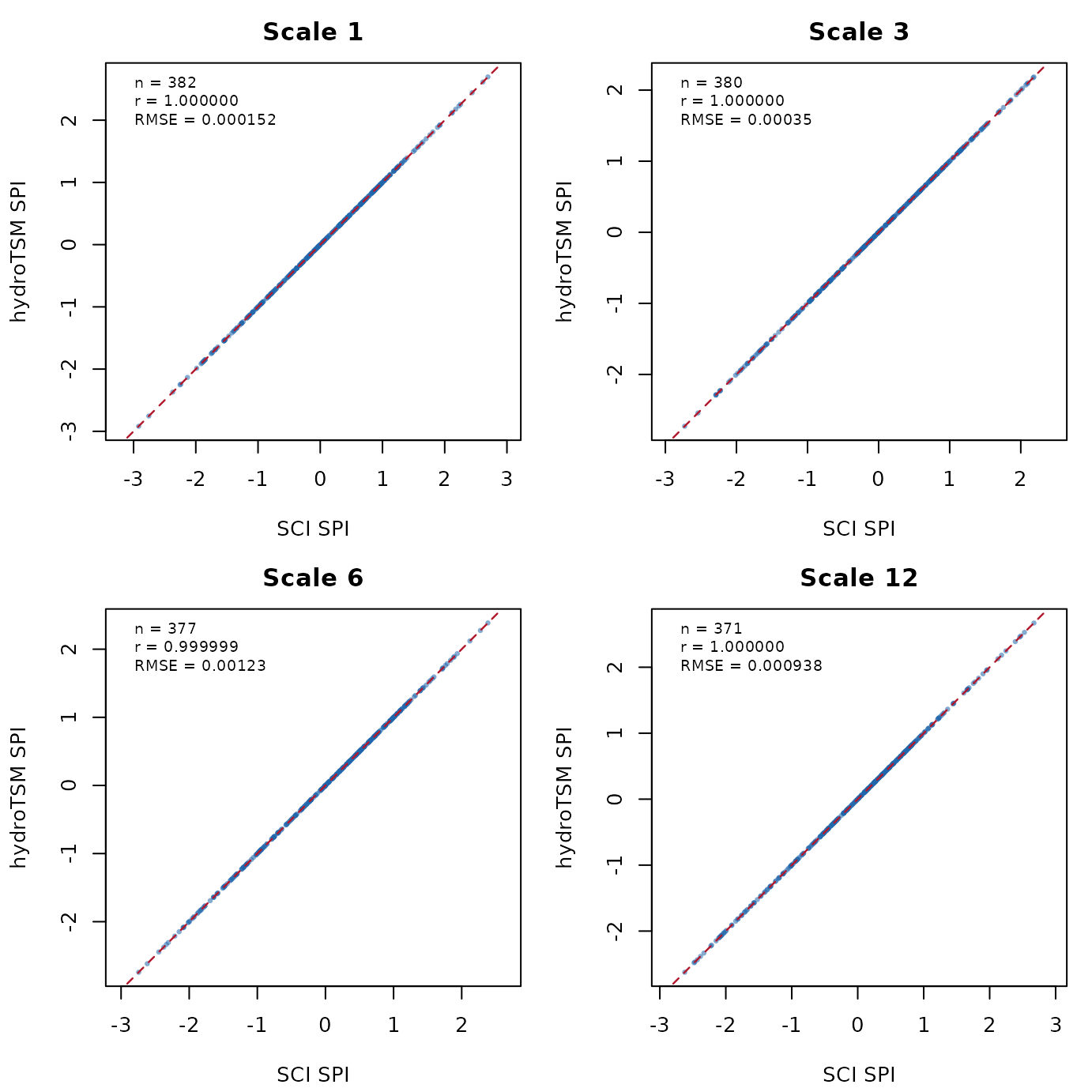
Figure 2. SPI: hydroTSM maximum likelihood versus SCI maximum likelihood.

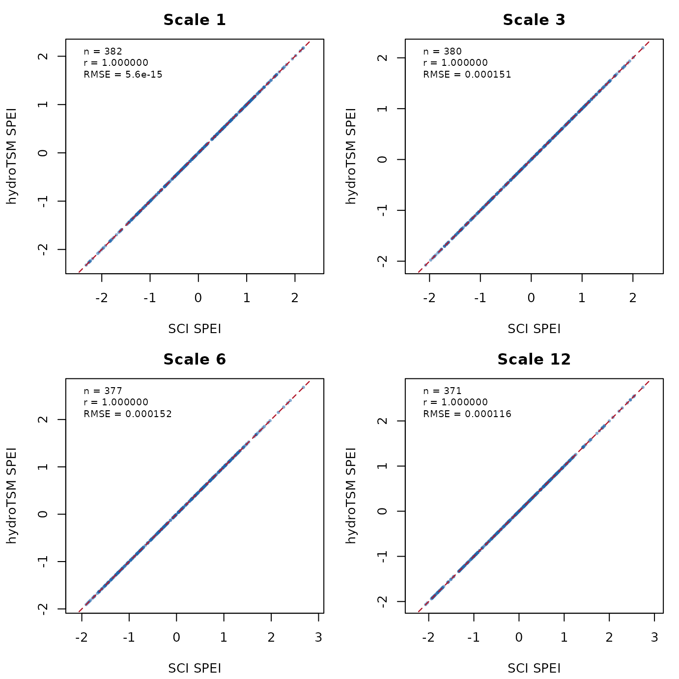
Figure 3. SPEI: hydroTSM maximum likelihood versus SCI maximum likelihood.

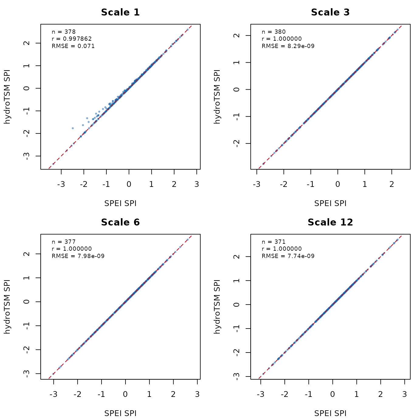
Figure 4. SPI: hydroTSM unbiased PWM versus the SPEI package. The scale-1 panel has different zero treatment.

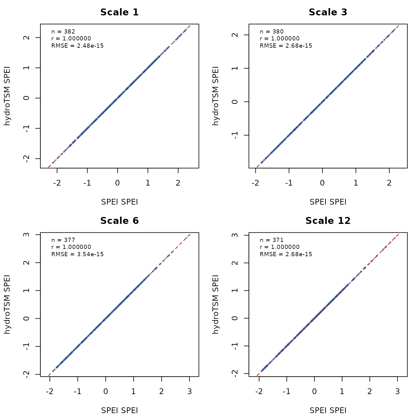
Figure 5. SPEI: hydroTSM unbiased PWM versus the SPEI package.

Interpretation

Under equivalent maximum-likelihood conditions, the largest RMSE against SCI was 0.001231 for SPI and 0.0001518 for SPEI. All correlations exceeded 0.99999926.

Under equivalent unbiased-PWM conditions, the largest RMSE against SPEI was 8.286e-09 for SPI at scales 3, 6, and 12, and 3.535e-15 for SPEI over all four scales. These differences are at or close to floating-point precision.

The direct scale-1 SPI comparison with SPEI had correlation 0.9978624 and RMSE 0.07103, but it is not a fair zero-treatment comparison. It must not be combined with the equivalent scale-3, scale-6, and scale-12 results when making a parity claim.

These results support two bounded conclusions for the tested data:

1. hydroTSM closely reproduces SCI when both use maximum likelihood, the same distributions, scaling, accumulation, and zero treatment; and
2. hydroTSM reproduces SPEI’s unbiased-PWM results when the distribution and zero treatment are equivalent.

They do not establish universal equality for other datasets, fitting failures, different reference periods, or intentionally different estimation methods.

Reproducing the external-package benchmark

The benchmark values are bundled so this vignette can be built without making SCI or SPEI package dependencies. A standalone script containing the complete external-package computation is installed with hydroTSM:

comparison.script <- system.file(
  "extdata", "compare_spi_spei.R.txt", package="hydroTSM"
)
source(comparison.script)

SCI, SPEI, and zoo must be installed to run that validation script. By default, it writes new compressed comparison and metadata CSV files to tempdir(). From the hydroTSM source directory, explicit output files can be supplied with:

Rscript inst/extdata/compare_spi_spei.R.txt values.csv.gz metadata.csv.gz

Because SCI and SPEI are comparison oracles rather than production dependencies, updating either package should be followed by regenerating the snapshot and reviewing all changes in finite-value coverage and accuracy.

References

McKee, T. B., Doesken, N. J., and Kleist, J. (1993). The relationship of drought frequency and duration to time scales. Proceedings of the 8th Conference on Applied Climatology, 179–184.

Guttman, N. B. (1998). Comparing the Palmer Drought Index and the Standardized Precipitation Index. Journal of the American Water Resources Association, 34, 113–121. doi:10.1111/j.1752-1688.1998.tb05964.x.

Hayes, M. J., Svoboda, M. D., Wilhite, D. A., and Vanyarkho, O. V. (1999). Monitoring the 1996 drought using the Standardized Precipitation Index. Bulletin of the American Meteorological Society, 80, 429–438.

Vicente-Serrano, S. M., Beguería, S., and López-Moreno, J. I. (2010). A multiscalar drought index sensitive to global warming: the Standardized Precipitation Evapotranspiration Index. Journal of Climate, 23, 1696–1718. doi:10.1175/2009JCLI2909.1.

Beguería, S., Vicente-Serrano, S. M., Reig, F., and Latorre, B. (2014). Standardized Precipitation Evapotranspiration Index (SPEI) revisited: parameter fitting, evapotranspiration models, tools, datasets and drought monitoring. International Journal of Climatology, 34, 3001–3023. doi:10.1002/joc.3887.

Greenwood, J. A., Landwehr, J. M., Matalas, N. C., and Wallis, J. R. (1979). Probability weighted moments: definition and relation to parameters of several distributions expressible in inverse form. Water Resources Research, 15, 1049–1054. doi:10.1029/WR015i005p01049.

Hosking, J. R. M. (1990). L-moments: analysis and estimation of distributions using linear combinations of order statistics. Journal of the Royal Statistical Society: Series B, 52, 105–124. doi:10.1111/j.2517-6161.1990.tb01775.x.

Stagge, J. H., Tallaksen, L. M., Gudmundsson, L., Van Loon, A. F., and Stahl, K. (2015). Candidate distributions for climatological drought indices (SPI and SPEI). International Journal of Climatology, 35, 4027–4040. doi:10.1002/joc.4267.

Pieper, P., Düsterhus, A., and Baehr, J. (2020). A universal Standardized Precipitation Index candidate distribution function for observations and simulations. Hydrology and Earth System Sciences, 24, 4541–4560. doi:10.5194/hess-24-4541-2020.