Pairwise dotty plots of parameter interactions coloured by objective-function performance

Creates a set of pairwise parameter plots for exploring how the objective function varies across the parameter space. For n selected parameters, the function generates sum(1:(npar-1)) plot_2parOF panels, corresponding to all possible two-parameter combinations.

Each panel displays one pair of parameters on the axes and colours the sampled parameter sets according to their goodness-of-fit values. This provides a compact visual summary of parameter sensitivity, equifinality, behavioural regions, and parameter interactions, which is especially useful in hydrological calibration studies based on Monte Carlo, PSO, GLUE, or other ensemble-based workflows.

Usage

plot_NparOF(params, gofs, param.names=colnames(params), 
         MinMax=c(NULL,"min","max"), beh.thr=NA, nrows="auto", 
         gof.name="GoF", main=paste(gof.name, "Surface"), GOFcuts="auto", 
         colorRamp= colorRampPalette(c("darkred", "red", "orange", "yellow", 
         "green", "darkgreen", "cyan")), points.cex=0.7, alpha=0.65, 
         axis.rot=c(0, 0), verbose=TRUE)

Arguments

params

matrix or data.frame with one row per parameter set and one column per model parameter.

gofs

numeric vector with the goodness-of-fit values associated with each row of params, in the same order. Therefore, length(gofs) must be equal to nrow(params).

param.names

character vector with the names of the parameters to be displayed. It can be a subset of colnames(params), allowing the user to focus on the parameters that are most relevant for a given hydrological analysis.

MinMax

character string indicating whether better model performance corresponds to minimising or maximising the objective function. Valid values are c(NULL, "min", "max"). This argument is required when beh.thr is used.

If MinMax="min", parameter sets with lower goodness-of-fit values are treated as better solutions and are plotted on top of poorer solutions. If MinMax="max", the opposite ordering is used. When MinMax=NULL, no preference for minimisation or maximisation is assumed.

beh.thr

optional numeric threshold used to retain only ‘behavioural’ parameter sets, following the GLUE terminology.

If MinMax="min", only parameter sets with gofs <= beh.thr are kept. If MinMax="max", only parameter sets with gofs >= beh.thr are kept. This is useful when the goal is to visualise only the acceptable region of the parameter space instead of the full ensemble.

nrows

numeric value giving the number of rows in the multi-panel plotting layout. If nrows="auto", the function computes the number of rows automatically from the number of panels to be produced.

gof.name

character string used as the title of the legend associated with the objective function values. Typical examples in hydrology are "NSE", "KGE", "RMSE", or "PBIAS".

main

character string intended for the main title. It is currently not used by the implementation.

GOFcuts

numeric vector defining the breakpoints used to convert gofs into performance classes for colouring the panels.

If GOFcuts="auto", the breakpoints are computed from quantiles of gofs. The quantile probabilities depend on MinMax:

if MinMax=NULL: probs = c(0, 0.1, 0.25, 0.5, 0.75, 0.9, 1)
if MinMax="min": probs = c(0, 0.25, 0.5, 0.85, 0.9, 0.97, 1)
if MinMax="max": probs = c(0, 0.03, 0.1, 0.15, 0.5, 0.75, 1)

Automatic breakpoints are convenient for highlighting performance gradients within large calibration ensembles.

colorRamp

function defining the colour ramp used to colour the points according to gofs, or a character vector with colours from which such a ramp can be built.

points.cex

numeric value controlling the size of the plotted points.

alpha

numeric value between 0 and 1 controlling colour transparency. 0 means fully transparent and 1 means fully opaque.

axis.rot

numeric vector of length 2 giving the rotation angles, in degrees, for the left or bottom and right or top axis labels, respectively.

verbose

logical value. If TRUE, progress messages are printed during filtering, breakpoint computation, and panel generation.

Value

Produces a lattice-based multi-panel figure on the active graphics device. Each panel is generated internally through plot_2parOF and shows one pairwise parameter projection coloured by objective-function performance. The final panel contains the legend for the goodness-of-fit classes.

This type of display is particularly useful for diagnosing parameter identifiability, interaction effects, trade-offs, and behavioural regions in hydrological model calibration.

Author

Mauricio Zambrano-Bigiarini, mzb.devel@gmail.com

Examples

# Number of dimensions to be optimised
D <- 5

# Boundaries of the search space (Rosenbrock test function)
lower <- rep(-30, D)
upper <- rep(30, D)

# \donttest{
local({
  
# Setting the user temporal directory as working directory
oldwd <- getwd()
on.exit(setwd(oldwd), add = TRUE)
setwd(tempdir())

# Setting the seed
set.seed(100)

# Optimising the Rosenbrock test function and writing the results to text files
hydroPSO(fn=rosenbrock, lower=lower, upper=upper,
         control=list(write2disk=TRUE))

# Reading the particle history generated by hydroPSO
particles <- read_particles(file="./PSO.out/Particles.txt", plot=FALSE)

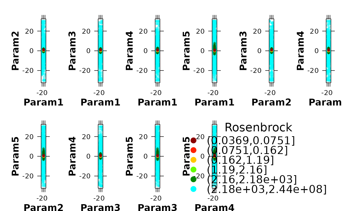
# Visualising pairwise parameter interactions coloured by model performance
plot_NparOF(params=particles[["part.params"]],
            gofs=particles[["part.gofs"]],
            gof.name="Rosenbrock",
            alpha=0.5)

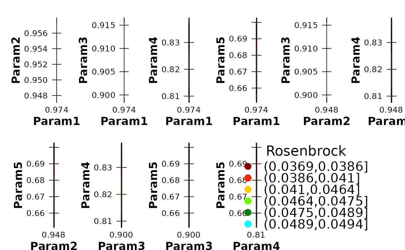
# Focusing only on behavioural parameter sets can help reveal
# the most plausible regions of the parameter space
thr <- quantile(particles[["part.gofs"]], probs=0.10, na.rm=TRUE)
plot_NparOF(params=particles[["part.params"]],
            gofs=particles[["part.gofs"]],
            MinMax="min", beh.thr=thr,
            gof.name="Rosenbrock",
            alpha=0.6)

}) # local END
#>                                                                                 
#> ================================================================================
#> [                                Initialising  ...                             ]
#> ================================================================================
#>                                                                                 
#> [npart=40 ; maxit=1000 ; method=spso2011 ; topology=random ; boundary.wall=absorbing2011]
#>          
#> [ user-definitions in control: write2disk=TRUE ]
#>          
#>                                                                                 
#> ================================================================================
#> [ Writing the 'PSO_logfile.txt' file ...                                       ]
#> ================================================================================
#>                                                                                 
#> ================================================================================
#> [                                 Running  PSO ...                             ]
#> ================================================================================
#>                                                                                 
#> iter: 100  Gbest: 1.953E+00  Gbest_rate:  1.15%  Iter_best_fit: 1.953E+00  nSwarm_Radius: 7.56E-04  |g-mean(p)|/mean(p):  8.88%
#> iter: 200  Gbest: 7.226E-01  Gbest_rate:  1.79%  Iter_best_fit: 7.226E-01  nSwarm_Radius: 2.36E-04  |g-mean(p)|/mean(p):  7.46%
#> iter: 300  Gbest: 3.295E-01  Gbest_rate:  0.45%  Iter_best_fit: 3.295E-01  nSwarm_Radius: 1.35E-04  |g-mean(p)|/mean(p):  6.39%
#> iter: 400  Gbest: 2.276E-01  Gbest_rate:  0.13%  Iter_best_fit: 2.276E-01  nSwarm_Radius: 2.18E-05  |g-mean(p)|/mean(p):  1.03%
#> iter: 500  Gbest: 1.556E-01  Gbest_rate:  0.18%  Iter_best_fit: 1.556E-01  nSwarm_Radius: 4.72E-05  |g-mean(p)|/mean(p):  3.32%
#> iter: 600  Gbest: 1.116E-01  Gbest_rate:  0.42%  Iter_best_fit: 1.116E-01  nSwarm_Radius: 4.51E-05  |g-mean(p)|/mean(p):  3.16%
#> iter: 700  Gbest: 8.683E-02  Gbest_rate:  0.26%  Iter_best_fit: 8.683E-02  nSwarm_Radius: 7.98E-05  |g-mean(p)|/mean(p):  3.16%
#> iter: 800  Gbest: 6.381E-02  Gbest_rate:  0.00%  Iter_best_fit: 6.384E-02  nSwarm_Radius: 3.68E-05  |g-mean(p)|/mean(p):  2.75%
#> iter: 900  Gbest: 4.697E-02  Gbest_rate:  0.86%  Iter_best_fit: 4.697E-02  nSwarm_Radius: 3.91E-05  |g-mean(p)|/mean(p):  4.31%
#> iter:1000  Gbest: 3.686E-02  Gbest_rate:  0.00%  Iter_best_fit: 3.689E-02  nSwarm_Radius: 1.16E-05  |g-mean(p)|/mean(p):  1.15%
#>                            
#> [ Writing output files... ]
#>                            
#>                                     |                                           
#> ================================================================================
#> [                          Creating the R output ...                           ]
#> ================================================================================
#>                                                      
#> [ Reading the file 'Particles.txt' ... ]
#> [ Total number of parameter sets: 40000 ]
#> [ Computed GOFcuts: 0.03686 0.07514 0.1619 1.191 2.156 2184 244200000 ]
#> [ Plotting 'Param1' vs 'Param2' ]
#> [ Plotting 'Param1' vs 'Param3' ]
#> [ Plotting 'Param1' vs 'Param4' ]
#> [ Plotting 'Param1' vs 'Param5' ]
#> [ Plotting 'Param2' vs 'Param3' ]
#> [ Plotting 'Param2' vs 'Param4' ]
#> [ Plotting 'Param2' vs 'Param5' ]
#> [ Plotting 'Param3' vs 'Param4' ]
#> [ Plotting 'Param3' vs 'Param5' ]
#> [ Plotting 'Param4' vs 'Param5' ]

#> [ Number of behavioural parameter sets: 4000 ]
#> [ Computed GOFcuts: 0.03686 0.03863 0.04095 0.04641 0.04748 0.04892 0.04944 ]
#> [ Plotting 'Param1' vs 'Param2' ]
#> [ Plotting 'Param1' vs 'Param3' ]
#> [ Plotting 'Param1' vs 'Param4' ]
#> [ Plotting 'Param1' vs 'Param5' ]
#> [ Plotting 'Param2' vs 'Param3' ]
#> [ Plotting 'Param2' vs 'Param4' ]
#> [ Plotting 'Param2' vs 'Param5' ]
#> [ Plotting 'Param3' vs 'Param4' ]
#> [ Plotting 'Param3' vs 'Param5' ]
#> [ Plotting 'Param4' vs 'Param5' ]

# } # donttest END